Abordemos las primeras ideas de regresión lineal a través de un ejemplo práctico:
Creamos dos variables, Ingreso y Consumo Esperado
import pandas as pd
import numpy as np
import matplotlib.pyplot as plt
import random
import statsmodels.formula.api as smf
from statsmodels.graphics.regressionplots import abline_plot


df = pd.DataFrame({
    'Col1': [1,2,3],
    'Col2': [4,5,6]
    })


familia = pd.DataFrame({'Y':[55,60,65,70,75,
                        65,70,74,80,85,88,
                        79,84,90,94,98,
                        80,93,95,103,108,113,115,
                        102,107,110,116,118,125,
                        110,115,120,130,135,140,
                        120,136,140,144,145,
                        135,137,140,152,157,160,162,
                        137,145,155,165,175,189,
                        150,152,175,178,180,185,191
                        ],'X':[80,80,80,80,80,
                   100,100,100,100,100,100,
                   120,120,120,120,120,
                   140,140,140,140,140,140,140,
                   160,160,160,160,160,160,
                   180,180,180,180,180,180,
                   200,200,200,200,200,
                   220,220,220,220,220,220,220,
                   240,240,240,240,240,240,
                   260,260,260,260,260,260,260
                   ]})
familia.head()ingresos = np.arange(80,261,20)
ingresos
consumoEsperado = [65,77,89,101,113,125,137,149,161,173]
consumoEsperado
familia.columnsIndex(['Y', 'X'], dtype='object')plt.figure() # llama al dispositivo grafico
plt.plot(ingresos,consumoEsperado)
plt.scatter(familia['X'],familia['Y'])
plt.show()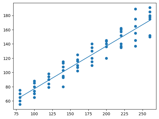
¿Qué hemos hecho?
¿Qué significa que sea lineal?
El término regresión lineal siempre significará una regresión lineal en los parámetros; los (es decir, los parámetros) se elevan sólo a la primera potencia. Puede o no ser lineal en las variables explicativas .
Para evidenciar la factibilidad del uso de RL en este caso, vamos a obtener una muestra de la población:
nS = familia.shape
type(nS)
indice = np.arange(0,nS[0])
indice # Creamos una variable indicadora para obtener una muestra
array([ 0, 1, 2, 3, 4, 5, 6, 7, 8, 9, 10, 11, 12, 13, 14, 15, 16,
17, 18, 19, 20, 21, 22, 23, 24, 25, 26, 27, 28, 29, 30, 31, 32, 33,
34, 35, 36, 37, 38, 39, 40, 41, 42, 43, 44, 45, 46, 47, 48, 49, 50,
51, 52, 53, 54, 55, 56, 57, 58, 59])random.seed(8519)
muestra = random.sample(list(indice),k = 20) # cambio de array a lista
muestra # samos sample para obtener una muestra sin reemplazo del tamaño indicado[54, 59, 33, 25, 32, 39, 47, 51, 18, 3, 34, 12, 29, 7, 26, 5, 56, 50, 44, 13]ingreso_muestra = familia.loc[muestra,'X']
consumo_muestra = familia.loc[muestra,'Y']df = pd.DataFrame(list(zip(consumo_muestra,ingreso_muestra)),columns = ['consumo_muestra','ingreso_muestra'])
ajuste_1 = smf.ols('consumo_muestra~ingreso_muestra',data =df).fit()
print(ajuste_1.summary()) OLS Regression Results
==============================================================================
Dep. Variable: consumo_muestra R-squared: 0.909
Model: OLS Adj. R-squared: 0.904
Method: Least Squares F-statistic: 179.4
Date: Wed, 18 Sep 2024 Prob (F-statistic): 8.44e-11
Time: 05:32:16 Log-Likelihood: -76.677
No. Observations: 20 AIC: 157.4
Df Residuals: 18 BIC: 159.3
Df Model: 1
Covariance Type: nonrobust
===================================================================================
coef std err t P>|t| [0.025 0.975]
-----------------------------------------------------------------------------------
Intercept 13.2650 8.817 1.504 0.150 -5.259 31.789
ingreso_muestra 0.6226 0.046 13.394 0.000 0.525 0.720
==============================================================================
Omnibus: 3.437 Durbin-Watson: 2.369
Prob(Omnibus): 0.179 Jarque-Bera (JB): 2.288
Skew: -0.828 Prob(JB): 0.319
Kurtosis: 2.997 Cond. No. 634.
==============================================================================
Notes:
[1] Standard Errors assume that the covariance matrix of the errors is correctly specified.
plt.figure()
plt.plot(df.ingreso_muestra,df.consumo_muestra,'o')
plt.plot(df.ingreso_muestra,ajuste_1.fittedvalues,'-',color='r')
plt.xlabel('Pcapincome')
plt.ylabel('Cellphone')
Regresión: Paso a paso
La función poblacional sería:
Como no es observable, se usa la muestral
Es por esto que los residuos se obtienen a través de los betas:
Diferenciando se obtiene:
donde
Abrimos la tabla3.2, vamos a obtener:
salario promedio por hora (Y) y
los años de escolaridad (X).
consumo = pd.read_csv('https://raw.githubusercontent.com/vmoprojs/DataLectures/master/GA/Tabla3_2.csv',
                      sep = ';',decimal = '.')


consumo.head()media_x = np.mean(consumo['X'])
media_y = np.mean(consumo['Y'])
n = consumo.shape[0]
sumcuad_x = np.sum(consumo['X']*consumo['X'])
sum_xy = np.sum(consumo['X']*consumo['Y'])
beta_som = (sum_xy-n*media_x*media_y)/(sumcuad_x-n*(media_x**2))
alpha_som = media_y-beta_som*media_x
(alpha_som,beta_som)(24.454545454545467, 0.509090909090909)Verificamos lo anterior mediante:
reg_1 = smf.ols('Y~X',data = consumo)
print(reg_1.fit().summary())
OLS Regression Results
==============================================================================
Dep. Variable: Y R-squared: 0.962
Model: OLS Adj. R-squared: 0.957
Method: Least Squares F-statistic: 202.9
Date: Wed, 18 Sep 2024 Prob (F-statistic): 5.75e-07
Time: 05:32:17 Log-Likelihood: -31.781
No. Observations: 10 AIC: 67.56
Df Residuals: 8 BIC: 68.17
Df Model: 1
Covariance Type: nonrobust
==============================================================================
coef std err t P>|t| [0.025 0.975]
------------------------------------------------------------------------------
Intercept 24.4545 6.414 3.813 0.005 9.664 39.245
X 0.5091 0.036 14.243 0.000 0.427 0.592
==============================================================================
Omnibus: 1.060 Durbin-Watson: 2.680
Prob(Omnibus): 0.589 Jarque-Bera (JB): 0.777
Skew: -0.398 Prob(JB): 0.678
Kurtosis: 1.891 Cond. No. 561.
==============================================================================
Notes:
[1] Standard Errors assume that the covariance matrix of the errors is correctly specified.
Veamos cómo queda nuestra estimación:
y_ajustado = alpha_som+beta_som*consumo['X']

dfAux = pd.DataFrame(list(zip(consumo['X'],y_ajustado)),
                     columns = ['X','y_ajustado'])
dfAuxe = consumo['Y']-y_ajustado
dfAux = pd.DataFrame(list(zip(consumo['X'],consumo['Y'],y_ajustado,e)),
columns = ['X','Y','y_ajustado','e'])
dfAuxnp.mean(e)
np.corrcoef(e,consumo['X'])array([[1.00000000e+00, 1.13838806e-15],
[1.13838806e-15, 1.00000000e+00]])SCT = np.sum((consumo['Y']-media_y)**2)
SCE = np.sum((y_ajustado-media_y)**2)
SCR = np.sum(e**2)
R_2 = SCE/SCT
R_2
0.9620615604867568print(reg_1.fit().summary()) OLS Regression Results
==============================================================================
Dep. Variable: Y R-squared: 0.962
Model: OLS Adj. R-squared: 0.957
Method: Least Squares F-statistic: 202.9
Date: Wed, 18 Sep 2024 Prob (F-statistic): 5.75e-07
Time: 05:32:17 Log-Likelihood: -31.781
No. Observations: 10 AIC: 67.56
Df Residuals: 8 BIC: 68.17
Df Model: 1
Covariance Type: nonrobust
==============================================================================
coef std err t P>|t| [0.025 0.975]
------------------------------------------------------------------------------
Intercept 24.4545 6.414 3.813 0.005 9.664 39.245
X 0.5091 0.036 14.243 0.000 0.427 0.592
==============================================================================
Omnibus: 1.060 Durbin-Watson: 2.680
Prob(Omnibus): 0.589 Jarque-Bera (JB): 0.777
Skew: -0.398 Prob(JB): 0.678
Kurtosis: 1.891 Cond. No. 561.
==============================================================================
Notes:
[1] Standard Errors assume that the covariance matrix of the errors is correctly specified.
Otro ejemplo
uu = 'https://raw.githubusercontent.com/vmoprojs/DataLectures/master/GA/table2_8.csv'

datos = pd.read_csv(uu,sep = ';')
datos.shape
datos.columns
m1 = smf.ols('FOODEXP~TOTALEXP',data = datos)
print(m1.fit().summary())
OLS Regression Results
==============================================================================
Dep. Variable: FOODEXP R-squared: 0.370
Model: OLS Adj. R-squared: 0.358
Method: Least Squares F-statistic: 31.10
Date: Wed, 18 Sep 2024 Prob (F-statistic): 8.45e-07
Time: 05:32:17 Log-Likelihood: -308.16
No. Observations: 55 AIC: 620.3
Df Residuals: 53 BIC: 624.3
Df Model: 1
Covariance Type: nonrobust
==============================================================================
coef std err t P>|t| [0.025 0.975]
------------------------------------------------------------------------------
Intercept 94.2088 50.856 1.852 0.070 -7.796 196.214
TOTALEXP 0.4368 0.078 5.577 0.000 0.280 0.594
==============================================================================
Omnibus: 0.763 Durbin-Watson: 2.083
Prob(Omnibus): 0.683 Jarque-Bera (JB): 0.258
Skew: 0.120 Prob(JB): 0.879
Kurtosis: 3.234 Cond. No. 3.66e+03
==============================================================================
Notes:
[1] Standard Errors assume that the covariance matrix of the errors is correctly specified.
[2] The condition number is large, 3.66e+03. This might indicate that there are
strong multicollinearity or other numerical problems.
Regresamos el gasto total en el gasto en alimentos
¿Son los coeficientes diferentes de cero?
import scipy.stats as st


t_ho = 0
t1 = (0.4368-t_ho)/ 0.078
(1-st.t.cdf(t1,df = 53))
3.8888077047438685e-07
t_ho = 0.3
t1 = (0.4368-t_ho)/ 0.078
(1-st.t.cdf(np.abs(t1),df = 53))0.04261898819196597Interpretación de los coeficientes
El coeficiente de la variable dependiente mide la tasa de cambio (derivada=pendiente) del modelo
La interpretación suele ser En promedio, el aumento de una unidad en la variable independiente produce un aumento/disminución de cantidad en la variable dependiente
Interprete la regresión anterior.
Práctica: Paridad del poder de compra
uu = "https://raw.githubusercontent.com/vmoprojs/DataLectures/master/GA/Tabla5_9.csv"

datos = pd.read_csv(uu,sep = ';')
datos.head()datos['EXCH'] = datos.EXCH.replace(to_replace= -99999, value=np.nan)
datos['PPP'] = datos.PPP.replace(to_replace = -99999, value = np.nan)
datos['LOCALC'] = datos.LOCALC.replace(to_replace= -99999, value = np.nan)
datos.head()Regresamos la paridad del poder de compra en la tasa de cambio
reg1 = smf.ols('EXCH~PPP',data = datos)
print(reg1.fit().summary())
OLS Regression Results
==============================================================================
Dep. Variable: EXCH R-squared: 0.987
Model: OLS Adj. R-squared: 0.986
Method: Least Squares F-statistic: 2066.
Date: Wed, 18 Sep 2024 Prob (F-statistic): 8.80e-28
Time: 05:32:17 Log-Likelihood: -205.44
No. Observations: 30 AIC: 414.9
Df Residuals: 28 BIC: 417.7
Df Model: 1
Covariance Type: nonrobust
==============================================================================
coef std err t P>|t| [0.025 0.975]
------------------------------------------------------------------------------
Intercept -61.3889 44.987 -1.365 0.183 -153.541 30.763
PPP 1.8153 0.040 45.450 0.000 1.733 1.897
==============================================================================
Omnibus: 35.744 Durbin-Watson: 2.062
Prob(Omnibus): 0.000 Jarque-Bera (JB): 94.065
Skew: -2.585 Prob(JB): 3.75e-21
Kurtosis: 9.966 Cond. No. 1.18e+03
==============================================================================
Notes:
[1] Standard Errors assume that the covariance matrix of the errors is correctly specified.
[2] The condition number is large, 1.18e+03. This might indicate that there are
strong multicollinearity or other numerical problems.
plt.figure()
plt.plot(np.arange(0,30),reg1.fit().resid,'-o')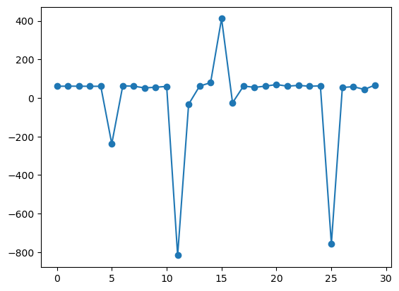
reg3 = smf.ols('np.log(EXCH)~np.log(PPP)',data = datos)
print(reg3.fit().summary())
OLS Regression Results
==============================================================================
Dep. Variable: np.log(EXCH) R-squared: 0.983
Model: OLS Adj. R-squared: 0.983
Method: Least Squares F-statistic: 1655.
Date: Wed, 18 Sep 2024 Prob (F-statistic): 1.87e-26
Time: 05:32:18 Log-Likelihood: -7.4056
No. Observations: 30 AIC: 18.81
Df Residuals: 28 BIC: 21.61
Df Model: 1
Covariance Type: nonrobust
===============================================================================
coef std err t P>|t| [0.025 0.975]
-------------------------------------------------------------------------------
Intercept 0.3436 0.086 3.990 0.000 0.167 0.520
np.log(PPP) 1.0023 0.025 40.688 0.000 0.952 1.053
==============================================================================
Omnibus: 2.829 Durbin-Watson: 1.629
Prob(Omnibus): 0.243 Jarque-Bera (JB): 1.449
Skew: -0.179 Prob(JB): 0.485
Kurtosis: 1.985 Cond. No. 5.38
==============================================================================
Notes:
[1] Standard Errors assume that the covariance matrix of the errors is correctly specified.
La PPA sostiene que con una unidad de moneda debe ser posible comprar la misma canasta de bienes en todos los países.
Práctica: Sueño
uu = "https://raw.githubusercontent.com/vmoprojs/DataLectures/master/WO/sleep75.csv"

datos = pd.read_csv(uu,sep = ",",header=None)
datos.columns
datos.columns = ["age","black","case","clerical","construc","educ","earns74","gdhlth","inlf", "leis1", "leis2", "leis3", "smsa", "lhrwage", "lothinc", "male", "marr", "prot", "rlxall", "selfe", "sleep", "slpnaps", "south", "spsepay", "spwrk75", "totwrk" , "union" , "worknrm" , "workscnd", "exper" , "yngkid","yrsmarr", "hrwage", "agesq"]
#totwrk: minutos trabajados por semana
# sleep: minutos dormidos por semana
plt.figure()
plt.scatter(datos['totwrk'],datos['sleep'])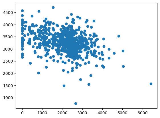
dormir = smf.ols('sleep~totwrk',data = datos)
print(dormir.fit().summary())
OLS Regression Results
==============================================================================
Dep. Variable: sleep R-squared: 0.103
Model: OLS Adj. R-squared: 0.102
Method: Least Squares F-statistic: 81.09
Date: Wed, 18 Sep 2024 Prob (F-statistic): 1.99e-18
Time: 05:32:18 Log-Likelihood: -5267.1
No. Observations: 706 AIC: 1.054e+04
Df Residuals: 704 BIC: 1.055e+04
Df Model: 1
Covariance Type: nonrobust
==============================================================================
coef std err t P>|t| [0.025 0.975]
------------------------------------------------------------------------------
Intercept 3586.3770 38.912 92.165 0.000 3509.979 3662.775
totwrk -0.1507 0.017 -9.005 0.000 -0.184 -0.118
==============================================================================
Omnibus: 68.651 Durbin-Watson: 1.955
Prob(Omnibus): 0.000 Jarque-Bera (JB): 192.044
Skew: -0.483 Prob(JB): 1.99e-42
Kurtosis: 5.365 Cond. No. 5.71e+03
==============================================================================
Notes:
[1] Standard Errors assume that the covariance matrix of the errors is correctly specified.
[2] The condition number is large, 5.71e+03. This might indicate that there are
strong multicollinearity or other numerical problems.
Para acceder a elementos de la estimación
print(dormir.fit().bse)
print(dormir.fit().params)
Intercept 38.912427
totwrk 0.016740
dtype: float64
Intercept 3586.376952
totwrk -0.150746
dtype: float64
Intervalo de confianza para y veamos los residuos
dormir.fit().params[1]+(-2*dormir.fit().bse[1],2*dormir.fit().bse[1])array([-0.18422633, -0.11726532])plt.figure()
plt.hist(dormir.fit().resid,bins = 60,density = True);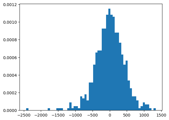
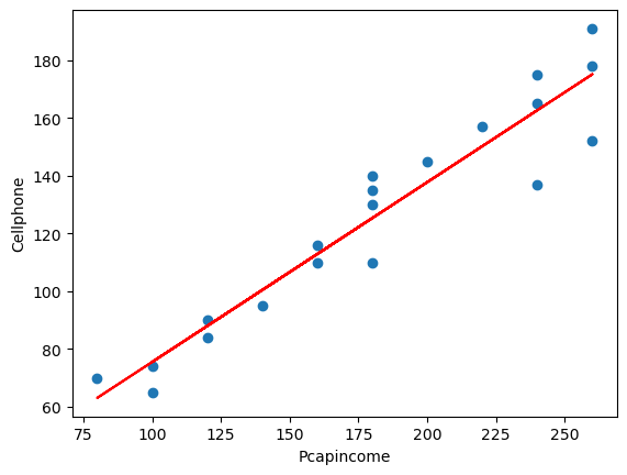
Transformaciones lineales
uu = "https://raw.githubusercontent.com/vmoprojs/DataLectures/master/GA/Table%2031_3.csv"

datos = pd.read_csv(uu, sep =';')

reg_1 = smf.ols('Cellphone~Pcapincome',data = datos)
print(reg_1.fit().summary())
OLS Regression Results
==============================================================================
Dep. Variable: Cellphone R-squared: 0.626
Model: OLS Adj. R-squared: 0.615
Method: Least Squares F-statistic: 53.67
Date: Wed, 18 Sep 2024 Prob (F-statistic): 2.50e-08
Time: 05:32:19 Log-Likelihood: -148.94
No. Observations: 34 AIC: 301.9
Df Residuals: 32 BIC: 304.9
Df Model: 1
Covariance Type: nonrobust
==============================================================================
coef std err t P>|t| [0.025 0.975]
------------------------------------------------------------------------------
Intercept 12.4795 6.109 2.043 0.049 0.037 24.922
Pcapincome 0.0023 0.000 7.326 0.000 0.002 0.003
==============================================================================
Omnibus: 1.398 Durbin-Watson: 2.381
Prob(Omnibus): 0.497 Jarque-Bera (JB): 0.531
Skew: 0.225 Prob(JB): 0.767
Kurtosis: 3.414 Cond. No. 3.46e+04
==============================================================================
Notes:
[1] Standard Errors assume that the covariance matrix of the errors is correctly specified.
[2] The condition number is large, 3.46e+04. This might indicate that there are
strong multicollinearity or other numerical problems.
plt.figure()
plt.plot(datos.Pcapincome,datos.Cellphone,'o')
plt.plot(datos.Pcapincome,reg_1.fit().fittedvalues,'-',color='r')
plt.xlabel('Pcapincome')
plt.ylabel('Cellphone')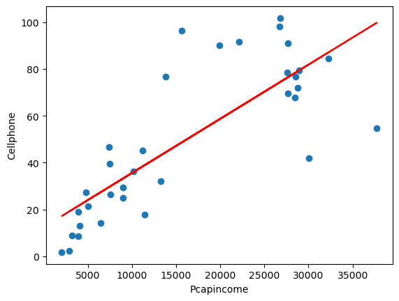
Modelo reciproco
uu =  "https://raw.githubusercontent.com/vmoprojs/DataLectures/master/GA/tabla_6_4.csv"
datos = pd.read_csv(uu,sep = ';')
datos.describe()plt.figure()
plt.plot(datos.PGNP,datos.CM,'o')
plt.xlabel('PGNP')
plt.ylabel('CM')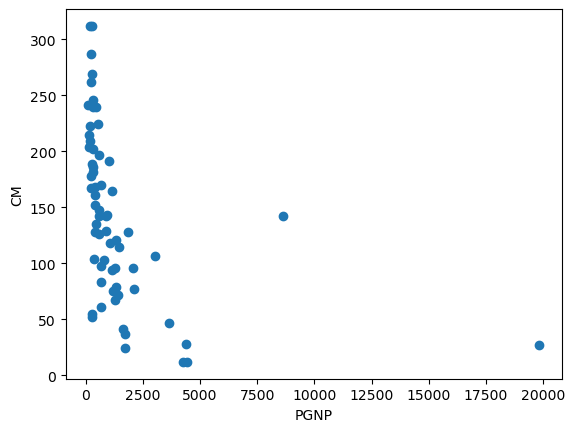
reg1 = smf.ols('CM~PGNP',data = datos)
print(reg1.fit().summary())
OLS Regression Results
==============================================================================
Dep. Variable: CM R-squared: 0.166
Model: OLS Adj. R-squared: 0.153
Method: Least Squares F-statistic: 12.36
Date: Wed, 18 Sep 2024 Prob (F-statistic): 0.000826
Time: 05:32:19 Log-Likelihood: -361.64
No. Observations: 64 AIC: 727.3
Df Residuals: 62 BIC: 731.6
Df Model: 1
Covariance Type: nonrobust
==============================================================================
coef std err t P>|t| [0.025 0.975]
------------------------------------------------------------------------------
Intercept 157.4244 9.846 15.989 0.000 137.743 177.105
PGNP -0.0114 0.003 -3.516 0.001 -0.018 -0.005
==============================================================================
Omnibus: 3.321 Durbin-Watson: 1.931
Prob(Omnibus): 0.190 Jarque-Bera (JB): 2.545
Skew: 0.345 Prob(JB): 0.280
Kurtosis: 2.309 Cond. No. 3.43e+03
==============================================================================
Notes:
[1] Standard Errors assume that the covariance matrix of the errors is correctly specified.
[2] The condition number is large, 3.43e+03. This might indicate that there are
strong multicollinearity or other numerical problems.
datos['RepPGNP'] = 1/datos.PGNP

reg2 = smf.ols('CM~RepPGNP',data = datos)
print(reg2.fit().summary())
OLS Regression Results
==============================================================================
Dep. Variable: CM R-squared: 0.459
Model: OLS Adj. R-squared: 0.450
Method: Least Squares F-statistic: 52.61
Date: Wed, 18 Sep 2024 Prob (F-statistic): 7.82e-10
Time: 05:32:20 Log-Likelihood: -347.79
No. Observations: 64 AIC: 699.6
Df Residuals: 62 BIC: 703.9
Df Model: 1
Covariance Type: nonrobust
==============================================================================
coef std err t P>|t| [0.025 0.975]
------------------------------------------------------------------------------
Intercept 81.7944 10.832 7.551 0.000 60.141 103.447
RepPGNP 2.727e+04 3759.999 7.254 0.000 1.98e+04 3.48e+04
==============================================================================
Omnibus: 0.147 Durbin-Watson: 1.959
Prob(Omnibus): 0.929 Jarque-Bera (JB): 0.334
Skew: 0.065 Prob(JB): 0.846
Kurtosis: 2.671 Cond. No. 534.
==============================================================================
Notes:
[1] Standard Errors assume that the covariance matrix of the errors is correctly specified.
Modelo log-lineal
uu = "https://raw.githubusercontent.com/vmoprojs/DataLectures/master/WO/ceosal2.csv"

datos = pd.read_csv(uu,header = None)
datos.columns = ["salary", "age", "college", "grad", "comten", "ceoten", "sales", "profits","mktval", "lsalary", "lsales", "lmktval", "comtensq", "ceotensq", "profmarg"]
datos.head()


reg1 = smf.ols('lsalary~ceoten',data = datos)
print(reg1.fit().summary())
OLS Regression Results
==============================================================================
Dep. Variable: lsalary R-squared: 0.013
Model: OLS Adj. R-squared: 0.008
Method: Least Squares F-statistic: 2.334
Date: Wed, 18 Sep 2024 Prob (F-statistic): 0.128
Time: 05:32:20 Log-Likelihood: -160.84
No. Observations: 177 AIC: 325.7
Df Residuals: 175 BIC: 332.0
Df Model: 1
Covariance Type: nonrobust
==============================================================================
coef std err t P>|t| [0.025 0.975]
------------------------------------------------------------------------------
Intercept 6.5055 0.068 95.682 0.000 6.371 6.640
ceoten 0.0097 0.006 1.528 0.128 -0.003 0.022
==============================================================================
Omnibus: 3.858 Durbin-Watson: 2.084
Prob(Omnibus): 0.145 Jarque-Bera (JB): 3.907
Skew: -0.189 Prob(JB): 0.142
Kurtosis: 3.622 Cond. No. 16.1
==============================================================================
Notes:
[1] Standard Errors assume that the covariance matrix of the errors is correctly specified.
Regresión a través del origen
uu = "https://raw.githubusercontent.com/vmoprojs/DataLectures/master/GA/Table%206_1.csv"
datos = pd.read_csv(uu,sep = ';')
datos.head()


lmod1 = smf.ols('Y~ -1+X',data = datos)
print(lmod1.fit().summary())
OLS Regression Results
=======================================================================================
Dep. Variable: Y R-squared (uncentered): 0.502
Model: OLS Adj. R-squared (uncentered): 0.500
Method: Least Squares F-statistic: 241.2
Date: Wed, 18 Sep 2024 Prob (F-statistic): 4.41e-38
Time: 05:32:21 Log-Likelihood: -751.30
No. Observations: 240 AIC: 1505.
Df Residuals: 239 BIC: 1508.
Df Model: 1
Covariance Type: nonrobust
==============================================================================
coef std err t P>|t| [0.025 0.975]
------------------------------------------------------------------------------
X 1.1555 0.074 15.532 0.000 1.009 1.302
==============================================================================
Omnibus: 9.576 Durbin-Watson: 1.973
Prob(Omnibus): 0.008 Jarque-Bera (JB): 13.569
Skew: -0.268 Prob(JB): 0.00113
Kurtosis: 4.034 Cond. No. 1.00
==============================================================================
Notes:
[1] R² is computed without centering (uncentered) since the model does not contain a constant.
[2] Standard Errors assume that the covariance matrix of the errors is correctly specified.
Regresión Lineal Múltiple
uu =  "https://raw.githubusercontent.com/vmoprojs/DataLectures/master/WO/hprice1.csv"
datos = pd.read_csv(uu,header=None)
datos.columns = ["price"   ,  "assess"  ,
                 "bdrms"  ,   "lotsize"  ,
                 "sqrft"   ,  "colonial",
                 "lprice"  ,  "lassess" ,
                 "llotsize" , "lsqrft"]

datos.describe()
modelo1 = smf.ols('lprice~lassess+llotsize+lsqrft+bdrms',data = datos)
print(modelo1.fit().summary())
OLS Regression Results
==============================================================================
Dep. Variable: lprice R-squared: 0.773
Model: OLS Adj. R-squared: 0.762
Method: Least Squares F-statistic: 70.58
Date: Wed, 18 Sep 2024 Prob (F-statistic): 6.45e-26
Time: 05:32:21 Log-Likelihood: 45.750
No. Observations: 88 AIC: -81.50
Df Residuals: 83 BIC: -69.11
Df Model: 4
Covariance Type: nonrobust
==============================================================================
coef std err t P>|t| [0.025 0.975]
------------------------------------------------------------------------------
Intercept 0.2637 0.570 0.463 0.645 -0.869 1.397
lassess 1.0431 0.151 6.887 0.000 0.742 1.344
llotsize 0.0074 0.039 0.193 0.848 -0.069 0.084
lsqrft -0.1032 0.138 -0.746 0.458 -0.379 0.172
bdrms 0.0338 0.022 1.531 0.129 -0.010 0.078
==============================================================================
Omnibus: 14.527 Durbin-Watson: 2.048
Prob(Omnibus): 0.001 Jarque-Bera (JB): 56.436
Skew: 0.118 Prob(JB): 5.56e-13
Kurtosis: 6.916 Cond. No. 501.
==============================================================================
Notes:
[1] Standard Errors assume that the covariance matrix of the errors is correctly specified.
modelo2 = smf.ols('lprice~llotsize+lsqrft+bdrms',data = datos)
print(modelo2.fit().summary())
OLS Regression Results
==============================================================================
Dep. Variable: lprice R-squared: 0.643
Model: OLS Adj. R-squared: 0.630
Method: Least Squares F-statistic: 50.42
Date: Wed, 18 Sep 2024 Prob (F-statistic): 9.74e-19
Time: 05:32:21 Log-Likelihood: 25.861
No. Observations: 88 AIC: -43.72
Df Residuals: 84 BIC: -33.81
Df Model: 3
Covariance Type: nonrobust
==============================================================================
coef std err t P>|t| [0.025 0.975]
------------------------------------------------------------------------------
Intercept -1.2970 0.651 -1.992 0.050 -2.592 -0.002
llotsize 0.1680 0.038 4.388 0.000 0.092 0.244
lsqrft 0.7002 0.093 7.540 0.000 0.516 0.885
bdrms 0.0370 0.028 1.342 0.183 -0.018 0.092
==============================================================================
Omnibus: 12.060 Durbin-Watson: 2.089
Prob(Omnibus): 0.002 Jarque-Bera (JB): 34.890
Skew: -0.188 Prob(JB): 2.65e-08
Kurtosis: 6.062 Cond. No. 410.
==============================================================================
Notes:
[1] Standard Errors assume that the covariance matrix of the errors is correctly specified.
modelo3 = smf.ols('lprice~bdrms',data = datos)
print(modelo3.fit().summary())
OLS Regression Results
==============================================================================
Dep. Variable: lprice R-squared: 0.215
Model: OLS Adj. R-squared: 0.206
Method: Least Squares F-statistic: 23.53
Date: Wed, 18 Sep 2024 Prob (F-statistic): 5.43e-06
Time: 05:32:21 Log-Likelihood: -8.8147
No. Observations: 88 AIC: 21.63
Df Residuals: 86 BIC: 26.58
Df Model: 1
Covariance Type: nonrobust
==============================================================================
coef std err t P>|t| [0.025 0.975]
------------------------------------------------------------------------------
Intercept 5.0365 0.126 39.862 0.000 4.785 5.288
bdrms 0.1672 0.034 4.851 0.000 0.099 0.236
==============================================================================
Omnibus: 7.476 Durbin-Watson: 2.056
Prob(Omnibus): 0.024 Jarque-Bera (JB): 13.085
Skew: -0.182 Prob(JB): 0.00144
Kurtosis: 4.854 Cond. No. 17.2
==============================================================================
Notes:
[1] Standard Errors assume that the covariance matrix of the errors is correctly specified.
import seaborn as sns

sns.pairplot(datos.loc[:,['lprice','llotsize' , 'lsqrft' , 'bdrms']])
<seaborn.axisgrid.PairGrid at 0x7fae51a15ca0>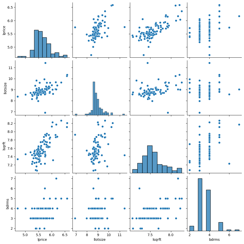
Predicción
datos_nuevos = pd.DataFrame({'llotsize':np.log(2100),'lsqrft':np.log(8000),'bdrms':4},index = [0])

pred_vals = modelo2.fit().predict()
modelo2.fit().get_prediction().summary_frame().head()pred_vals = modelo2.fit().get_prediction(datos_nuevos)
pred_vals.summary_frame()RLM: Educación con insumos
uu = "https://raw.githubusercontent.com/vmoprojs/DataLectures/master/WO/gpa1.csv"
datosgpa = pd.read_csv(uu, header = None)
datosgpa.columns = ["age",  "soph",  "junior",    "senior",    "senior5",  "male", "campus",   "business", "engineer", "colGPA",   "hsGPA",    "ACT",  "job19",    "job20",    "drive",    "bike", "walk", "voluntr",  "PC",   "greek",    "car",  "siblings", "bgfriend", "clubs",    "skipped",  "alcohol",  "gradMI",   "fathcoll", "mothcoll"]

reg4 = smf.ols('colGPA ~ PC', data = datosgpa)
print(reg4.fit().summary())
OLS Regression Results
==============================================================================
Dep. Variable: colGPA R-squared: 0.050
Model: OLS Adj. R-squared: 0.043
Method: Least Squares F-statistic: 7.314
Date: Wed, 18 Sep 2024 Prob (F-statistic): 0.00770
Time: 05:32:25 Log-Likelihood: -56.641
No. Observations: 141 AIC: 117.3
Df Residuals: 139 BIC: 123.2
Df Model: 1
Covariance Type: nonrobust
==============================================================================
coef std err t P>|t| [0.025 0.975]
------------------------------------------------------------------------------
Intercept 2.9894 0.040 75.678 0.000 2.911 3.068
PC 0.1695 0.063 2.704 0.008 0.046 0.293
==============================================================================
Omnibus: 2.136 Durbin-Watson: 1.941
Prob(Omnibus): 0.344 Jarque-Bera (JB): 1.852
Skew: 0.160 Prob(JB): 0.396
Kurtosis: 2.539 Cond. No. 2.45
==============================================================================
Notes:
[1] Standard Errors assume that the covariance matrix of the errors is correctly specified.
reg5 = smf.ols('colGPA ~ PC + hsGPA + ACT', data = datosgpa)
print(reg5.fit().summary())
OLS Regression Results
==============================================================================
Dep. Variable: colGPA R-squared: 0.219
Model: OLS Adj. R-squared: 0.202
Method: Least Squares F-statistic: 12.83
Date: Wed, 18 Sep 2024 Prob (F-statistic): 1.93e-07
Time: 05:32:25 Log-Likelihood: -42.796
No. Observations: 141 AIC: 93.59
Df Residuals: 137 BIC: 105.4
Df Model: 3
Covariance Type: nonrobust
==============================================================================
coef std err t P>|t| [0.025 0.975]
------------------------------------------------------------------------------
Intercept 1.2635 0.333 3.793 0.000 0.605 1.922
PC 0.1573 0.057 2.746 0.007 0.044 0.271
hsGPA 0.4472 0.094 4.776 0.000 0.262 0.632
ACT 0.0087 0.011 0.822 0.413 -0.012 0.029
==============================================================================
Omnibus: 2.770 Durbin-Watson: 1.870
Prob(Omnibus): 0.250 Jarque-Bera (JB): 1.863
Skew: 0.016 Prob(JB): 0.394
Kurtosis: 2.438 Cond. No. 298.
==============================================================================
Notes:
[1] Standard Errors assume that the covariance matrix of the errors is correctly specified.