2. Pandas

2.1. Las Series

import pandas as pd
#pd.Series?

animales = ['Tigre', 'Oso', 'Alce']
pd.Series(animales)

0    Tigre
1      Oso
2     Alce
dtype: object

animales = ['Tigre', 'Oso', None]
pd.Series(animales)

0    Tigre
1      Oso
2     None
dtype: object

numbers = [1, 2, None]
pd.Series(numbers)

0    1.0
1    2.0
2    NaN
dtype: float64

import numpy as np
np.nan == None

False

np.nan == np.nan

False

np.isnan(np.nan)

True

sports = {'Futbol': 'Ecuador',
          'Golf': 'Escocia',
          'Sumo': 'Japon',
          'Taekwondo': 'Corea del Sur'}
s = pd.Series(sports)
s

Futbol             Ecuador
Golf               Escocia
Sumo                 Japon
Taekwondo    Corea del Sur
dtype: object

s.index

Index(['Futbol', 'Golf', 'Sumo', 'Taekwondo'], dtype='object')

s = pd.Series(['Tigre', 'Oso', 'Alce'], index=['India', 'America', 'Canada'])
s

India      Tigre
America      Oso
Canada      Alce
dtype: object

sports = {'Futbol': 'Ecuador',
          'Golf': 'Escocia',
          'Sumo': 'Japon',
          'Taekwondo': 'Corea del Sur'}
s = pd.Series(sports, index=['Golf', 'Sumo', 'Hockey'])
s

Golf      Escocia
Sumo        Japon
Hockey        NaN
dtype: object

2.2. Haciendo consultas en Series

sports = {'Futbol': 'Ecuador',
          'Golf': 'Escocia',
          'Sumo': 'Japon',
          'Taekwondo': 'Corea del Sur'}
s = pd.Series(sports)
s

Futbol             Ecuador
Golf               Escocia
Sumo                 Japon
Taekwondo    Corea del Sur
dtype: object

s.iloc[3]

'Corea del Sur'

s.loc['Golf']

'Escocia'

s[3]

'Corea del Sur'

s['Golf']

'Escocia'

sports = {99: 'Ecuador',
          100: 'Escocia',
          101: 'Japon',
          102: 'Corea del Sur'}
s = pd.Series(sports)

#  s[0] # no se hace la consulta

s = pd.Series([100.00, 120.00, 101.00, 3.00])
s

0    100.0
1    120.0
2    101.0
3      3.0
dtype: float64

total = 0
for item in s:
    total+=item
print(total)

324.0

s = pd.Series([1, 2, 3])
s.loc['Animal'] = 'Bears' # agregamos un elemento a la serie
s

0             1
1             2
2             3
Animal    Bears
dtype: object

2.3. Pandas: estructuras de datos para estadística

Provee estructuras de datos adecuados para análisis estadístico, y añade funciones que facilitan el ingreso de datos, su organización y su manipulación.

2.3.1. Manipulación de datos

Procedimientos comunes

Un DataFrame es una estructura de datos de dos dimensiones con etiquetas cuyas columnas pueden ser de diferentes tipos.

Empecemos creando un DataFrame con tres columnas Time, x y y

import numpy as np
import pandas as pd

t = np.arange(0,10,0.1)
x = np.sin(t)
y = np.cos(t)

df = pd.DataFrame({'Time':t, 'x':x,'y':y})

En pandas las filas se referencian por índices y las columnas por nombres. Si si desea la primera columna se tiene dos opciones:

df.Time
df['Time']

0     0.0
1     0.1
2     0.2
3     0.3
4     0.4
     ... 
95    9.5
96    9.6
97    9.7
98    9.8
99    9.9
Name: Time, Length: 100, dtype: float64

Si se desea extraer más de una columna, se lo hace con una lista:

data = df[['Time','x']]

Para despleguar las primeras o últimas filas tenemos:

data.head()
data.tail()

	Time	x
95	9.5	-0.075151
96	9.6	-0.174327
97	9.7	-0.271761
98	9.8	-0.366479
99	9.9	-0.457536

Para extraer las filas de la 5 a la 10 tenemos:

data[4:10]

	Time	x
4	0.4	0.389418
5	0.5	0.479426
6	0.6	0.564642
7	0.7	0.644218
8	0.8	0.717356
9	0.9	0.783327

El manejo de DataFrames es un tanto diferente de arrays en numpy. Por ejemplo, filas (enumeradas) y columnas (etiquetadas) se acceden de forma simultánea de la siguiente manera:

df[['Time','y']][4:10]

	Time	y
4	0.4	0.921061
5	0.5	0.877583
6	0.6	0.825336
7	0.7	0.764842
8	0.8	0.696707
9	0.9	0.621610

También se puede usar la manera estándar de fila/columna usando iloc:

df.iloc[4:10,[0,2]]

	Time	y
4	0.4	0.921061
5	0.5	0.877583
6	0.6	0.825336
7	0.7	0.764842
8	0.8	0.696707
9	0.9	0.621610

Finalmente, a veces se desea tener acceso directo a los datos, no al DataFrame, se usa:

# df.values

Lo que devuelve un numpy array

Notas en Selección de datos

Es cierto que DataFrames y arrays son parecidos, pero sus filosofías son diferentes. Es bueno tener muy claro sus diferencias para acceder a los datos:

• numpy: maneja filas primero. Ej., data[0] es la primera fila del array

• pandas: empieza con columnas. Ej., df['values'][0] es el primer elemento de la columna values.

Si un DataFrame tiene filas con etiquetas, puedes por ejemplo extraer la fila rowlabel con df.loc['rowlabel']. Si quieres acceder con el número de la fila, se hace con df.iloc[15]. También puedes usar iloc para acceder a datos en formato fila/columna df.ioc[2:4,3]

Extraer filas también funciona, por ejemplo df[0:5] para las primeras 5 filas. Lo que suele ser confuso es que para extraer una única fila se usa por ejmeplo df[5:6]. Si usas solo df[5] se devuelve un error.

2.3.2. Agrupaciones

pandas ofrece funciones poderosas para manejar datos perdidos que suelen ser reemplazados por nan (not a number). También permite realizar manipilaciones más sofisticadas como pivotaje. Por ejemplo, se puede usar DataFrames para hacer grupos y su análisis estadístico de cada grupo.

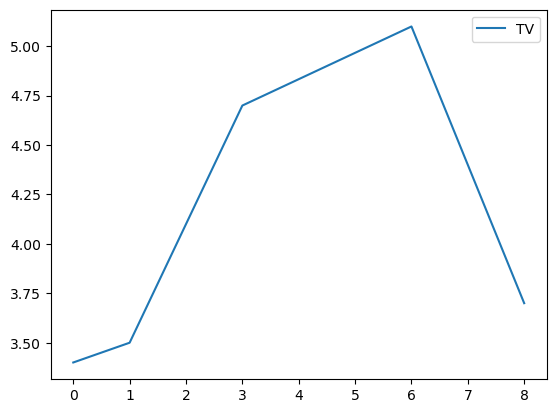
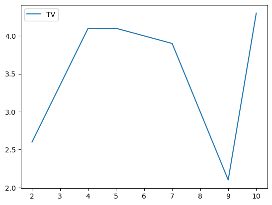
Veamos este ejemplo de datos del número de horas que la gente ve televisión agrupado por m y f.

import pandas as pd
import numpy as np

data = pd.DataFrame({
    'Gender' : ['f', 'f', 'm', 'f', 'm','m', 'f', 'm', 'f', 'm', 'm'], 
    'TV': [3.4, 3.5, 2.6, 4.7, 4.1, 4.1, 5.1, 3.9, 3.7, 2.1, 4.3]
})

data

	Gender	TV
0	f	3.4
1	f	3.5
2	m	2.6
3	f	4.7
4	m	4.1
5	m	4.1
6	f	5.1
7	m	3.9
8	f	3.7
9	m	2.1
10	m	4.3

#Agrupamos los datos

grouped = data.groupby('Gender')
grouped.apply(print)

  Gender   TV
0      f  3.4
1      f  3.5
3      f  4.7
6      f  5.1
8      f  3.7
   Gender   TV
2       m  2.6
4       m  4.1
5       m  4.1
7       m  3.9
9       m  2.1
10      m  4.3

# Algunas estadísticas generales
grouped.describe()

	TV
	count	mean	std	min	25%	50%	75%	max
Gender
f	5.0	4.080000	0.769415	3.4	3.500	3.7	4.7	5.1
m	6.0	3.516667	0.926103	2.1	2.925	4.0	4.1	4.3

# Graficamos los datos
grouped.plot()

Gender
f    Axes(0.125,0.11;0.775x0.77)
m    Axes(0.125,0.11;0.775x0.77)
dtype: object

# Separamos los grupos como DataFrames
df_female = grouped.get_group('f')
df_female

	Gender	TV
0	f	3.4
1	f	3.5
3	f	4.7
6	f	5.1
8	f	3.7

# Obtenemos los datos como un numpy-array
values_female = df_female.values
values_female

array([['f', 3.4],
       ['f', 3.5],
       ['f', 4.7],
       ['f', 5.1],
       ['f', 3.7]], dtype=object)

2.3.3. Merge

import pandas as pd

df = pd.DataFrame([{'Name': 'Chris', 'Item Purchased': 'Sponge', 'Cost': 22.50},
                   {'Name': 'Kevyn', 'Item Purchased': 'Kitty Litter', 'Cost': 2.50},
                   {'Name': 'Filip', 'Item Purchased': 'Spoon', 'Cost': 5.00}],
                  index=['Store 1', 'Store 1', 'Store 2'])
df

	Name	Item Purchased	Cost
Store 1	Chris	Sponge	22.5
Store 1	Kevyn	Kitty Litter	2.5
Store 2	Filip	Spoon	5.0

df['Date'] = ['December 1', 'January 1', 'mid-May']
df

	Name	Item Purchased	Cost	Date
Store 1	Chris	Sponge	22.5	December 1
Store 1	Kevyn	Kitty Litter	2.5	January 1
Store 2	Filip	Spoon	5.0	mid-May

df['Delivered'] = True
df

	Name	Item Purchased	Cost	Date	Delivered
Store 1	Chris	Sponge	22.5	December 1	True
Store 1	Kevyn	Kitty Litter	2.5	January 1	True
Store 2	Filip	Spoon	5.0	mid-May	True

df['Feedback'] = ['Positive', None, 'Negative']
df

	Name	Item Purchased	Cost	Date	Delivered	Feedback
Store 1	Chris	Sponge	22.5	December 1	True	Positive
Store 1	Kevyn	Kitty Litter	2.5	January 1	True	None
Store 2	Filip	Spoon	5.0	mid-May	True	Negative

adf = df.reset_index()
adf['Date'] = pd.Series({0: 'December 1', 2: 'mid-May'})
adf

	index	Name	Item Purchased	Cost	Date	Delivered	Feedback
0	Store 1	Chris	Sponge	22.5	December 1	True	Positive
1	Store 1	Kevyn	Kitty Litter	2.5	NaN	True	None
2	Store 2	Filip	Spoon	5.0	mid-May	True	Negative

staff_df = pd.DataFrame([{'Name': 'Kelly', 'Role': 'Director of HR'},
                         {'Name': 'Sally', 'Role': 'Course liasion'},
                         {'Name': 'James', 'Role': 'Grader'}])
staff_df = staff_df.set_index('Name')
student_df = pd.DataFrame([{'Name': 'James', 'School': 'Business'},
                           {'Name': 'Mike', 'School': 'Law'},
                           {'Name': 'Sally', 'School': 'Engineering'}])
student_df = student_df.set_index('Name')
print(staff_df.head())
print()
print(student_df.head())

                 Role
Name                 
Kelly  Director of HR
Sally  Course liasion
James          Grader

            School
Name              
James     Business
Mike           Law
Sally  Engineering

Tipos de join

pd.merge(staff_df, student_df, how='outer', left_index=True, right_index=True)

	Role	School
Name
James	Grader	Business
Kelly	Director of HR	NaN
Mike	NaN	Law
Sally	Course liasion	Engineering

pd.merge(staff_df, student_df, how='inner', left_index=True, right_index=True)

	Role	School
Name
Sally	Course liasion	Engineering
James	Grader	Business

pd.merge(staff_df, student_df, how='left', left_index=True, right_index=True)

	Role	School
Name
Kelly	Director of HR	NaN
Sally	Course liasion	Engineering
James	Grader	Business

pd.merge(staff_df, student_df, how='right', left_index=True, right_index=True)

	Role	School
Name
James	Grader	Business
Mike	NaN	Law
Sally	Course liasion	Engineering

staff_df = staff_df.reset_index()
student_df = student_df.reset_index()
pd.merge(staff_df, student_df, how='left', left_on='Name', right_on='Name')

	Name	Role	School
0	Kelly	Director of HR	NaN
1	Sally	Course liasion	Engineering
2	James	Grader	Business

staff_df = pd.DataFrame([{'Name': 'Kelly', 'Role': 'Director of HR', 'Location': 'State Street'},
                         {'Name': 'Sally', 'Role': 'Course liasion', 'Location': 'Washington Avenue'},
                         {'Name': 'James', 'Role': 'Grader', 'Location': 'Washington Avenue'}])
student_df = pd.DataFrame([{'Name': 'James', 'School': 'Business', 'Location': '1024 Billiard Avenue'},
                           {'Name': 'Mike', 'School': 'Law', 'Location': 'Fraternity House #22'},
                           {'Name': 'Sally', 'School': 'Engineering', 'Location': '512 Wilson Crescent'}])
pd.merge(staff_df, student_df, how='left', left_on='Name', right_on='Name')

	Name	Role	Location_x	School	Location_y
0	Kelly	Director of HR	State Street	NaN	NaN
1	Sally	Course liasion	Washington Avenue	Engineering	512 Wilson Crescent
2	James	Grader	Washington Avenue	Business	1024 Billiard Avenue

staff_df = pd.DataFrame([{'First Name': 'Kelly', 'Last Name': 'Desjardins', 'Role': 'Director of HR'},
                         {'First Name': 'Sally', 'Last Name': 'Brooks', 'Role': 'Course liasion'},
                         {'First Name': 'James', 'Last Name': 'Wilde', 'Role': 'Grader'}])
student_df = pd.DataFrame([{'First Name': 'James', 'Last Name': 'Hammond', 'School': 'Business'},
                           {'First Name': 'Mike', 'Last Name': 'Smith', 'School': 'Law'},
                           {'First Name': 'Sally', 'Last Name': 'Brooks', 'School': 'Engineering'}])
staff_df
student_df
pd.merge(staff_df, student_df, how='inner', left_on=['First Name','Last Name'], right_on=['First Name','Last Name'])

	First Name	Last Name	Role	School
0	Sally	Brooks	Course liasion	Engineering

2.3.4. Datos categóricos

df = pd.DataFrame(['A+', 'A', 'A-', 'B+', 'B', 'B-', 'C+', 'C', 'C-', 'D+', 'D'],
                  index=['excellent', 'excellent', 'excellent', 'good', 'good', 'good', 'ok', 'ok', 'ok', 'poor', 'poor'])
df.rename(columns={0: 'Grades'}, inplace=True)
df

	Grades
excellent	A+
excellent	A
excellent	A-
good	B+
good	B
good	B-
ok	C+
ok	C
ok	C-
poor	D+
poor	D

df['Grades'].astype('category').head()

excellent    A+
excellent     A
excellent    A-
good         B+
good          B
Name: Grades, dtype: category
Categories (11, object): ['A', 'A+', 'A-', 'B', ..., 'C+', 'C-', 'D', 'D+']

grades = pd.Categorical(df.Grades, categories=['D', 'D+', 'C-', 'C', 'C+', 'B-', 'B', 'B+', 'A-', 'A', 'A+'],
                              ordered=True)
grades

['A+', 'A', 'A-', 'B+', 'B', ..., 'C+', 'C', 'C-', 'D+', 'D']
Length: 11
Categories (11, object): ['D' < 'D+' < 'C-' < 'C' ... 'B+' < 'A-' < 'A' < 'A+']

grades > 'C'

array([ True,  True,  True,  True,  True,  True,  True, False, False,
       False, False])

#import os as os
#os.chdir("C:/Users/VICTOR/Documents/AnalyticsPython/Data")
df = pd.read_csv('https://raw.githubusercontent.com/vmoprojs/DataLectures/master/census.csv')
df = df[df['SUMLEV']==50]
df = df.set_index('STNAME').groupby(level=0)['CENSUS2010POP'].agg([np.average]).rename(columns={'average': 'avg'})
pd.cut(df['avg'],10)

STNAME
Alabama                   (11706.087, 75333.413]
Alaska                    (11706.087, 75333.413]
Arizona                 (390320.176, 453317.529]
Arkansas                  (11706.087, 75333.413]
California              (579312.234, 642309.586]
Colorado                 (75333.413, 138330.766]
Connecticut             (390320.176, 453317.529]
Delaware                (264325.471, 327322.823]
District of Columbia    (579312.234, 642309.586]
Florida                 (264325.471, 327322.823]
Georgia                   (11706.087, 75333.413]
Hawaii                  (264325.471, 327322.823]
Idaho                     (11706.087, 75333.413]
Illinois                 (75333.413, 138330.766]
Indiana                   (11706.087, 75333.413]
Iowa                      (11706.087, 75333.413]
Kansas                    (11706.087, 75333.413]
Kentucky                  (11706.087, 75333.413]
Louisiana                 (11706.087, 75333.413]
Maine                    (75333.413, 138330.766]
Maryland                (201328.118, 264325.471]
Massachusetts           (453317.529, 516314.881]
Michigan                 (75333.413, 138330.766]
Minnesota                 (11706.087, 75333.413]
Mississippi               (11706.087, 75333.413]
Missouri                  (11706.087, 75333.413]
Montana                   (11706.087, 75333.413]
Nebraska                  (11706.087, 75333.413]
Nevada                  (138330.766, 201328.118]
New Hampshire            (75333.413, 138330.766]
New Jersey              (390320.176, 453317.529]
New Mexico                (11706.087, 75333.413]
New York                (264325.471, 327322.823]
North Carolina           (75333.413, 138330.766]
North Dakota              (11706.087, 75333.413]
Ohio                     (75333.413, 138330.766]
Oklahoma                  (11706.087, 75333.413]
Oregon                   (75333.413, 138330.766]
Pennsylvania            (138330.766, 201328.118]
Rhode Island            (201328.118, 264325.471]
South Carolina           (75333.413, 138330.766]
South Dakota              (11706.087, 75333.413]
Tennessee                 (11706.087, 75333.413]
Texas                    (75333.413, 138330.766]
Utah                     (75333.413, 138330.766]
Vermont                   (11706.087, 75333.413]
Virginia                  (11706.087, 75333.413]
Washington              (138330.766, 201328.118]
West Virginia             (11706.087, 75333.413]
Wisconsin                (75333.413, 138330.766]
Wyoming                   (11706.087, 75333.413]
Name: avg, dtype: category
Categories (10, interval[float64, right]): [(11706.087, 75333.413] < (75333.413, 138330.766] < (138330.766, 201328.118] < (201328.118, 264325.471] ... (390320.176, 453317.529] < (453317.529, 516314.881] < (516314.881, 579312.234] < (579312.234, 642309.586]]

2.3.5. Tablas dinámicas

uu = "https://raw.githubusercontent.com/vmoprojs/DataLectures/master/cars.csv"
df = pd.read_csv(uu)
df.describe()

	YEAR	(kW)	CITY (kWh/100 km)	HWY (kWh/100 km)	COMB (kWh/100 km)	CITY (Le/100 km)	HWY (Le/100 km)	COMB (Le/100 km)	(g/km)	RATING	(km)	TIME (h)
count	53.000000	53.000000	53.00000	53.000000	53.000000	53.000000	53.000000	53.000000	53.0	19.0	53.000000	53.000000
mean	2014.735849	190.622642	19.64717	21.633962	20.541509	2.207547	2.422642	2.301887	0.0	10.0	239.169811	8.471698
std	1.227113	155.526429	3.00100	1.245753	1.979455	0.344656	0.143636	0.212576	0.0	0.0	141.426352	2.991036
min	2012.000000	35.000000	15.20000	18.800000	16.800000	1.700000	2.100000	1.900000	0.0	10.0	100.000000	4.000000
25%	2014.000000	80.000000	17.00000	20.800000	18.700000	1.900000	2.300000	2.100000	0.0	10.0	117.000000	7.000000
50%	2015.000000	107.000000	19.00000	21.700000	20.000000	2.100000	2.400000	2.200000	0.0	10.0	135.000000	8.000000
75%	2016.000000	283.000000	22.40000	22.500000	22.100000	2.500000	2.500000	2.500000	0.0	10.0	402.000000	12.000000
max	2016.000000	568.000000	23.90000	23.300000	23.600000	2.700000	2.600000	2.600000	0.0	10.0	473.000000	12.000000

df.head()

	YEAR	Make	Model	Size	(kW)	Unnamed: 5	TYPE	CITY (kWh/100 km)	HWY (kWh/100 km)	COMB (kWh/100 km)	CITY (Le/100 km)	HWY (Le/100 km)	COMB (Le/100 km)	(g/km)	RATING	(km)	TIME (h)
0	2012	MITSUBISHI	i-MiEV	SUBCOMPACT	49	A1	B	16.9	21.4	18.7	1.9	2.4	2.1	0	NaN	100	7
1	2012	NISSAN	LEAF	MID-SIZE	80	A1	B	19.3	23.0	21.1	2.2	2.6	2.4	0	NaN	117	7
2	2013	FORD	FOCUS ELECTRIC	COMPACT	107	A1	B	19.0	21.1	20.0	2.1	2.4	2.2	0	NaN	122	4
3	2013	MITSUBISHI	i-MiEV	SUBCOMPACT	49	A1	B	16.9	21.4	18.7	1.9	2.4	2.1	0	NaN	100	7
4	2013	NISSAN	LEAF	MID-SIZE	80	A1	B	19.3	23.0	21.1	2.2	2.6	2.4	0	NaN	117	7

df.pivot_table(values='(kW)', index='YEAR', columns='Make', aggfunc=np.mean)

Make	BMW	CHEVROLET	FORD	KIA	MITSUBISHI	NISSAN	SMART	TESLA
YEAR
2012	NaN	NaN	NaN	NaN	49.0	80.0	NaN	NaN
2013	NaN	NaN	107.0	NaN	49.0	80.0	35.0	280.000000
2014	NaN	104.0	107.0	NaN	49.0	80.0	35.0	268.333333
2015	125.0	104.0	107.0	81.0	49.0	80.0	35.0	320.666667
2016	125.0	104.0	107.0	81.0	49.0	80.0	35.0	409.700000

df.pivot_table(values='(kW)', index='YEAR', columns='Make', aggfunc=[np.mean,np.min], margins=True)

	mean									amin
Make	BMW	CHEVROLET	FORD	KIA	MITSUBISHI	NISSAN	SMART	TESLA	All	BMW	CHEVROLET	FORD	KIA	MITSUBISHI	NISSAN	SMART	TESLA	All
YEAR
2012	NaN	NaN	NaN	NaN	49.0	80.0	NaN	NaN	64.500000	NaN	NaN	NaN	NaN	49.0	80.0	NaN	NaN	49
2013	NaN	NaN	107.0	NaN	49.0	80.0	35.0	280.000000	158.444444	NaN	NaN	107.0	NaN	49.0	80.0	35.0	270.0	35
2014	NaN	104.0	107.0	NaN	49.0	80.0	35.0	268.333333	135.000000	NaN	104.0	107.0	NaN	49.0	80.0	35.0	225.0	35
2015	125.0	104.0	107.0	81.0	49.0	80.0	35.0	320.666667	181.428571	125.0	104.0	107.0	81.0	49.0	80.0	35.0	280.0	35
2016	125.0	104.0	107.0	81.0	49.0	80.0	35.0	409.700000	252.263158	125.0	104.0	107.0	81.0	49.0	80.0	35.0	283.0	35
All	125.0	104.0	107.0	81.0	49.0	80.0	35.0	345.478261	190.622642	125.0	104.0	107.0	81.0	49.0	80.0	35.0	225.0	35