6. Regresión lineal#
Abordemos las primeras ideas de regresión lineal a través de un ejemplo práctico:
Creamos dos variables, Ingreso y Consumo Esperado
import pandas as pd
import numpy as np
import matplotlib.pyplot as plt
import random
import statsmodels.formula.api as stm
from statsmodels.graphics.regressionplots import abline_plot


df = pd.DataFrame({
    'Col1': [1,2,3],
    'Col2': [4,5,6]
    })


familia = pd.DataFrame({'Y':[55,60,65,70,75,
                        65,70,74,80,85,88,
                        79,84,90,94,98,
                        80,93,95,103,108,113,115,
                        102,107,110,116,118,125,
                        110,115,120,130,135,140,
                        120,136,140,144,145,
                        135,137,140,152,157,160,162,
                        137,145,155,165,175,189,
                        150,152,175,178,180,185,191
                        ],'X':[80,80,80,80,80,
                   100,100,100,100,100,100,
                   120,120,120,120,120,
                   140,140,140,140,140,140,140,
                   160,160,160,160,160,160,
                   180,180,180,180,180,180,
                   200,200,200,200,200,
                   220,220,220,220,220,220,220,
                   240,240,240,240,240,240,
                   260,260,260,260,260,260,260
                   ]})
familia.head()
| Y | X | |
|---|---|---|
| 0 | 55 | 80 |
| 1 | 60 | 80 |
| 2 | 65 | 80 |
| 3 | 70 | 80 |
| 4 | 75 | 80 |
ingresos = np.arange(80,261,20)
ingresos
consumoEsperado = [65,77,89,101,113,125,137,149,161,173]
consumoEsperado


familia.columns
Index(['Y', 'X'], dtype='object')
plt.figure() # llama al dispositivo grafico
plt.plot(ingresos,consumoEsperado)
plt.scatter(familia['X'],familia['Y'])
plt.show()
¿Qué hemos hecho?
¿Qué significa que sea lineal?
El término regresión lineal siempre significará una regresión lineal en los parámetros; los \(\beta\) (es decir, los parámetros) se elevan sólo a la primera potencia. Puede o no ser lineal en las variables explicativas \(X\).
Para evidenciar la factibilidad del uso de RL en este caso, vamos a obtener una muestra de la población:
nS = familia.shape
type(nS)
indice = np.arange(0,nS[0])
indice # Creamos una variable indicadora para obtener una muestra
array([ 0,  1,  2,  3,  4,  5,  6,  7,  8,  9, 10, 11, 12, 13, 14, 15, 16,
       17, 18, 19, 20, 21, 22, 23, 24, 25, 26, 27, 28, 29, 30, 31, 32, 33,
       34, 35, 36, 37, 38, 39, 40, 41, 42, 43, 44, 45, 46, 47, 48, 49, 50,
       51, 52, 53, 54, 55, 56, 57, 58, 59])
random.seed(8519)
muestra = random.sample(list(indice),k = 20) # cambio de array a lista
muestra # samos sample para obtener una muestra sin reemplazo del tamaño indicado
[54, 59, 33, 25, 32, 39, 47, 51, 18, 3, 34, 12, 29, 7, 26, 5, 56, 50, 44, 13]
ingreso_muestra = familia.loc[muestra,'X']
consumo_muestra = familia.loc[muestra,'Y']
df = pd.DataFrame(list(zip(consumo_muestra,ingreso_muestra)),columns = ['consumo_muestra','ingreso_muestra'])
ajuste_1 = stm.ols('consumo_muestra~ingreso_muestra',data =df).fit()

print(ajuste_1.summary())
                            OLS Regression Results
==============================================================================
Dep. Variable:        consumo_muestra   R-squared:                       0.909
Model:                            OLS   Adj. R-squared:                  0.904
Method:                 Least Squares   F-statistic:                     179.4
Date:                Wed, 16 Apr 2025   Prob (F-statistic):           8.44e-11
Time:                        04:04:54   Log-Likelihood:                -76.677
No. Observations:                  20   AIC:                             157.4
Df Residuals:                      18   BIC:                             159.3
Df Model:                           1
Covariance Type:            nonrobust
===================================================================================
                      coef    std err          t      P>|t|      [0.025      0.975]
-----------------------------------------------------------------------------------
Intercept          13.2650      8.817      1.504      0.150      -5.259      31.789
ingreso_muestra     0.6226      0.046     13.394      0.000       0.525       0.720
==============================================================================
Omnibus:                        3.437   Durbin-Watson:                   2.369
Prob(Omnibus):                  0.179   Jarque-Bera (JB):                2.288
Skew:                          -0.828   Prob(JB):                        0.319
Kurtosis:                       2.997   Cond. No.                         634.
==============================================================================

Notes:
[1] Standard Errors assume that the covariance matrix of the errors is correctly specified.
plt.figure()
plt.plot(df.ingreso_muestra,df.consumo_muestra,'o')
plt.plot(df.ingreso_muestra,ajuste_1.fittedvalues,'-',color='r')
plt.xlabel('Pcapincome')
plt.ylabel('Cellphone')
Text(0, 0.5, 'Cellphone')
6.1. Regresión: Paso a paso#
La función poblacional sería:
Como no es observable, se usa la muestral
Es por esto que los residuos se obtienen a través de los betas:
Diferenciando se obtiene:
donde
Abrimos la tabla3.2, vamos a obtener:
salario promedio por hora (Y) y
los años de escolaridad (X).
consumo = pd.read_csv('https://raw.githubusercontent.com/vmoprojs/DataLectures/master/GA/Tabla3_2.csv',
                      sep = ';',decimal = '.')


consumo.head()
| Y | X | |
|---|---|---|
| 0 | 70 | 80 |
| 1 | 65 | 100 |
| 2 | 90 | 120 |
| 3 | 95 | 140 |
| 4 | 110 | 160 |
media_x = np.mean(consumo['X'])
media_y = np.mean(consumo['Y'])


n = consumo.shape[0]

sumcuad_x = np.sum(consumo['X']*consumo['X'])
sum_xy = np.sum(consumo['X']*consumo['Y'])

beta_som = (sum_xy-n*media_x*media_y)/(sumcuad_x-n*(media_x**2))
alpha_som = media_y-beta_som*media_x
(alpha_som,beta_som)
(24.454545454545467, 0.509090909090909)
Verificamos lo anterior mediante:
reg_1 = stm.ols('Y~X',data = consumo)
print(reg_1.fit().summary())
                            OLS Regression Results
==============================================================================
Dep. Variable:                      Y   R-squared:                       0.962
Model:                            OLS   Adj. R-squared:                  0.957
Method:                 Least Squares   F-statistic:                     202.9
Date:                Wed, 16 Apr 2025   Prob (F-statistic):           5.75e-07
Time:                        04:04:55   Log-Likelihood:                -31.781
No. Observations:                  10   AIC:                             67.56
Df Residuals:                       8   BIC:                             68.17
Df Model:                           1
Covariance Type:            nonrobust
==============================================================================
                 coef    std err          t      P>|t|      [0.025      0.975]
------------------------------------------------------------------------------
Intercept     24.4545      6.414      3.813      0.005       9.664      39.245
X              0.5091      0.036     14.243      0.000       0.427       0.592
==============================================================================
Omnibus:                        1.060   Durbin-Watson:                   2.680
Prob(Omnibus):                  0.589   Jarque-Bera (JB):                0.777
Skew:                          -0.398   Prob(JB):                        0.678
Kurtosis:                       1.891   Cond. No.                         561.
==============================================================================

Notes:
[1] Standard Errors assume that the covariance matrix of the errors is correctly specified.
/Users/victormorales/opt/anaconda3/lib/python3.9/site-packages/scipy/stats/_stats_py.py:1806: UserWarning: kurtosistest only valid for n>=20 ... continuing anyway, n=10
  warnings.warn("kurtosistest only valid for n>=20 ... continuing "
Veamos cómo queda nuestra estimación:
y_ajustado = alpha_som+beta_som*consumo['X']

dfAux = pd.DataFrame(list(zip(consumo['X'],y_ajustado)),
                     columns = ['X','y_ajustado'])
dfAux
| X | y_ajustado | |
|---|---|---|
| 0 | 80 | 65.181818 |
| 1 | 100 | 75.363636 |
| 2 | 120 | 85.545455 |
| 3 | 140 | 95.727273 |
| 4 | 160 | 105.909091 |
| 5 | 180 | 116.090909 |
| 6 | 200 | 126.272727 |
| 7 | 220 | 136.454545 |
| 8 | 240 | 146.636364 |
| 9 | 260 | 156.818182 |
e = consumo['Y']-y_ajustado


dfAux = pd.DataFrame(list(zip(consumo['X'],consumo['Y'],y_ajustado,e)),
                     columns = ['X','Y','y_ajustado','e'])

dfAux
| X | Y | y_ajustado | e | |
|---|---|---|---|---|
| 0 | 80 | 70 | 65.181818 | 4.818182 |
| 1 | 100 | 65 | 75.363636 | -10.363636 |
| 2 | 120 | 90 | 85.545455 | 4.454545 |
| 3 | 140 | 95 | 95.727273 | -0.727273 |
| 4 | 160 | 110 | 105.909091 | 4.090909 |
| 5 | 180 | 115 | 116.090909 | -1.090909 |
| 6 | 200 | 120 | 126.272727 | -6.272727 |
| 7 | 220 | 140 | 136.454545 | 3.545455 |
| 8 | 240 | 155 | 146.636364 | 8.363636 |
| 9 | 260 | 150 | 156.818182 | -6.818182 |
np.mean(e)
np.corrcoef(e,consumo['X'])
array([[1.00000000e+00, 1.13838806e-15],
       [1.13838806e-15, 1.00000000e+00]])
SCT = np.sum((consumo['Y']-media_y)**2)
SCE = np.sum((y_ajustado-media_y)**2)
SCR = np.sum(e**2)

R_2 = SCE/SCT
R_2
0.9620615604867568
print(reg_1.fit().summary())
                            OLS Regression Results
==============================================================================
Dep. Variable:                      Y   R-squared:                       0.962
Model:                            OLS   Adj. R-squared:                  0.957
Method:                 Least Squares   F-statistic:                     202.9
Date:                Wed, 16 Apr 2025   Prob (F-statistic):           5.75e-07
Time:                        04:04:55   Log-Likelihood:                -31.781
No. Observations:                  10   AIC:                             67.56
Df Residuals:                       8   BIC:                             68.17
Df Model:                           1
Covariance Type:            nonrobust
==============================================================================
                 coef    std err          t      P>|t|      [0.025      0.975]
------------------------------------------------------------------------------
Intercept     24.4545      6.414      3.813      0.005       9.664      39.245
X              0.5091      0.036     14.243      0.000       0.427       0.592
==============================================================================
Omnibus:                        1.060   Durbin-Watson:                   2.680
Prob(Omnibus):                  0.589   Jarque-Bera (JB):                0.777
Skew:                          -0.398   Prob(JB):                        0.678
Kurtosis:                       1.891   Cond. No.                         561.
==============================================================================

Notes:
[1] Standard Errors assume that the covariance matrix of the errors is correctly specified.
/Users/victormorales/opt/anaconda3/lib/python3.9/site-packages/scipy/stats/_stats_py.py:1806: UserWarning: kurtosistest only valid for n>=20 ... continuing anyway, n=10
  warnings.warn("kurtosistest only valid for n>=20 ... continuing "
[Ejemplo 2.3] Salario del CEO y retorno sobre el capital
\(y\): Salario anual en miles de dólares
\(x\): Retorno sobre el capital (ROE) promedio de la firma en los últimos 3 años.
uu = "https://raw.githubusercontent.com/vmoprojs/DataLectures/master/WO/ceosal1.csv"
datos = pd.read_csv(uu)
datos.columns = ["salary","pcsalary" ,"sales", "roe","pcroe","ros","indus","finance",
                "consprod" ,"utility" , "lsalary" , "lsales"  ]
reg_ceosal1 = stm.ols('salary~roe',data = datos)
print(reg_ceosal1.fit().summary())
                            OLS Regression Results
==============================================================================
Dep. Variable:                 salary   R-squared:                       0.013
Model:                            OLS   Adj. R-squared:                  0.008
Method:                 Least Squares   F-statistic:                     2.767
Date:                Wed, 16 Apr 2025   Prob (F-statistic):             0.0978
Time:                        04:04:56   Log-Likelihood:                -1804.5
No. Observations:                 209   AIC:                             3613.
Df Residuals:                     207   BIC:                             3620.
Df Model:                           1
Covariance Type:            nonrobust
==============================================================================
                 coef    std err          t      P>|t|      [0.025      0.975]
------------------------------------------------------------------------------
Intercept    963.1913    213.240      4.517      0.000     542.790    1383.592
roe           18.5012     11.123      1.663      0.098      -3.428      40.431
==============================================================================
Omnibus:                      311.096   Durbin-Watson:                   2.105
Prob(Omnibus):                  0.000   Jarque-Bera (JB):            31120.902
Skew:                           6.915   Prob(JB):                         0.00
Kurtosis:                      61.158   Cond. No.                         43.3
==============================================================================

Notes:
[1] Standard Errors assume that the covariance matrix of the errors is correctly specified.
Si \(roe=0\), el salario predicho es igual al intercepto, USD \(963.191,00\).
Si el \(roe\) aumenta un punto porcentual, \(\Delta roe=1\), entonces el salario cambia USD \(18.500,00\)
Como la ecuación es lineal, este resultado no depende del salario inicial.
[Ejemplo 2.4] Salario y Educación
\(y\): Salario, medido en dólares por hora.
\(x\): años de educación.
uu = "https://raw.githubusercontent.com/vmoprojs/DataLectures/master/WO/wage1.csv"
datos = pd.read_csv(uu)
datos.columns = ["wage"  ,   "educ"   ,  "exper"  ,  "tenure"  , "nonwhite", "female"  , "married" , "numdep",
                "smsa"  ,   "northcen" ,"south" ,   "west" ,    "construc" ,"ndurman" , "trcommpu" ,"trade",
                "services" ,"profserv", "profocc" , "clerocc" , "servocc"  ,"lwage" ,   "expersq" , "tenursq" ]
reg_sal = stm.ols("wage~educ",data = datos)
print(reg_sal.fit().summary())
                            OLS Regression Results
==============================================================================
Dep. Variable:                   wage   R-squared:                       0.164
Model:                            OLS   Adj. R-squared:                  0.163
Method:                 Least Squares   F-statistic:                     102.9
Date:                Wed, 16 Apr 2025   Prob (F-statistic):           3.44e-22
Time:                        04:04:57   Log-Likelihood:                -1383.4
No. Observations:                 525   AIC:                             2771.
Df Residuals:                     523   BIC:                             2779.
Df Model:                           1
Covariance Type:            nonrobust
==============================================================================
                 coef    std err          t      P>|t|      [0.025      0.975]
------------------------------------------------------------------------------
Intercept     -0.8916      0.686     -1.300      0.194      -2.239       0.456
educ           0.5406      0.053     10.143      0.000       0.436       0.645
==============================================================================
Omnibus:                      211.871   Durbin-Watson:                   1.825
Prob(Omnibus):                  0.000   Jarque-Bera (JB):              803.455
Skew:                           1.859   Prob(JB):                    3.40e-175
Kurtosis:                       7.787   Cond. No.                         60.2
==============================================================================

Notes:
[1] Standard Errors assume that the covariance matrix of the errors is correctly specified.
En promedio, un año más de educación genera un aumento de 0.5406 dólares más en el salsario por ahora.
[Ejemplo 2.5] Resultados de la votación y gastos de campaña
\(y\): \(voteA\), es el porcentaje de voto recibido por el candidato A.
\(x\): \(shareA\) es el porcentaje del total de campaña gastado por el candidato A.
uu = "https://raw.githubusercontent.com/vmoprojs/DataLectures/master/WO/vote1.csv"
datos = pd.read_csv(uu)
datos.columns = ["state"    ,"district", "democA",   "voteA" ,   "expendA" , "expendB",  "prtystrA" ,"lexpendA",
                "lexpendB" ,"shareA"  ]
reg_vote = stm.ols("voteA~shareA",data = datos)
print(reg_vote.fit().summary())
                            OLS Regression Results
==============================================================================
Dep. Variable:                  voteA   R-squared:                       0.856
Model:                            OLS   Adj. R-squared:                  0.855
Method:                 Least Squares   F-statistic:                     1018.
Date:                Wed, 16 Apr 2025   Prob (F-statistic):           6.63e-74
Time:                        04:04:57   Log-Likelihood:                -565.20
No. Observations:                 173   AIC:                             1134.
Df Residuals:                     171   BIC:                             1141.
Df Model:                           1
Covariance Type:            nonrobust
==============================================================================
                 coef    std err          t      P>|t|      [0.025      0.975]
------------------------------------------------------------------------------
Intercept     26.8122      0.887     30.221      0.000      25.061      28.564
shareA         0.4638      0.015     31.901      0.000       0.435       0.493
==============================================================================
Omnibus:                       20.747   Durbin-Watson:                   1.826
Prob(Omnibus):                  0.000   Jarque-Bera (JB):               44.613
Skew:                           0.525   Prob(JB):                     2.05e-10
Kurtosis:                       5.255   Cond. No.                         112.
==============================================================================

Notes:
[1] Standard Errors assume that the covariance matrix of the errors is correctly specified.
Esto significa que si la proporción del gasto del candidato A aumenta en un punto porcentual, el candidato \(A\) recibe casi medio punto porcentual (\(0,464\)) más del voto total.
En algunos casos, el análisis de regresión no se utiliza para determinar la causalidad, sino simplemente para observar si dos variables están relacionadas positiva o negativamente, de forma muy similar a un análisis de correlación estándar.
6.1.1. Incorporando no linealidades en la regresión simple#
uu = "https://raw.githubusercontent.com/vmoprojs/DataLectures/master/WO/wage1.csv"
datos = pd.read_csv(uu)
datos.columns = ["wage"  ,   "educ"   ,  "exper"  ,  "tenure"  , "nonwhite", "female"  , "married" , "numdep",
                "smsa"  ,   "northcen" ,"south" ,   "west" ,    "construc" ,"ndurman" , "trcommpu" ,"trade",
                "services" ,"profserv", "profocc" , "clerocc" , "servocc"  ,"lwage" ,   "expersq" , "tenursq" ]
reg_wage = stm.ols("lwage~educ",data  = datos)
print(reg_wage.fit().summary())
                            OLS Regression Results
==============================================================================
Dep. Variable:                  lwage   R-squared:                       0.185
Model:                            OLS   Adj. R-squared:                  0.184
Method:                 Least Squares   F-statistic:                     119.0
Date:                Wed, 16 Apr 2025   Prob (F-statistic):           4.19e-25
Time:                        04:04:57   Log-Likelihood:                -358.91
No. Observations:                 525   AIC:                             721.8
Df Residuals:                     523   BIC:                             730.3
Df Model:                           1
Covariance Type:            nonrobust
==============================================================================
                 coef    std err          t      P>|t|      [0.025      0.975]
------------------------------------------------------------------------------
Intercept      0.5862      0.097      6.017      0.000       0.395       0.778
educ           0.0826      0.008     10.909      0.000       0.068       0.097
==============================================================================
Omnibus:                       11.629   Durbin-Watson:                   1.803
Prob(Omnibus):                  0.003   Jarque-Bera (JB):               13.615
Skew:                           0.265   Prob(JB):                      0.00111
Kurtosis:                       3.585   Cond. No.                         60.2
==============================================================================

Notes:
[1] Standard Errors assume that the covariance matrix of the errors is correctly specified.
El salario aumenta un 8,3% por cada año adicional de educación: el retorno de un año extra de educación.
Calcular
uu = "https://raw.githubusercontent.com/vmoprojs/DataLectures/master/WO/ceosal1.csv"
datos = pd.read_csv(uu)
datos.columns = ["salary","pcsalary" ,"sales", "roe","pcroe","ros","indus","finance",
                "consprod" ,"utility" , "lsalary" , "lsales"  ]
reg_ceolog = stm.ols("lsalary~lsales",data = datos)
print(reg_ceolog.fit().summary())
                            OLS Regression Results
==============================================================================
Dep. Variable:                lsalary   R-squared:                       0.211
Model:                            OLS   Adj. R-squared:                  0.207
Method:                 Least Squares   F-statistic:                     55.30
Date:                Wed, 16 Apr 2025   Prob (F-statistic):           2.70e-12
Time:                        04:04:58   Log-Likelihood:                -152.50
No. Observations:                 209   AIC:                             309.0
Df Residuals:                     207   BIC:                             315.7
Df Model:                           1
Covariance Type:            nonrobust
==============================================================================
                 coef    std err          t      P>|t|      [0.025      0.975]
------------------------------------------------------------------------------
Intercept      4.8220      0.288     16.723      0.000       4.254       5.390
lsales         0.2567      0.035      7.436      0.000       0.189       0.325
==============================================================================
Omnibus:                       84.151   Durbin-Watson:                   1.860
Prob(Omnibus):                  0.000   Jarque-Bera (JB):              403.831
Skew:                           1.507   Prob(JB):                     2.04e-88
Kurtosis:                       9.106   Cond. No.                         70.0
==============================================================================

Notes:
[1] Standard Errors assume that the covariance matrix of the errors is correctly specified.
El coeficiente de \(log(ventas)\) es la elasticidad estimada del salario con respecto a las ventas. Implica que un aumento del \(1\%\) en las ventas de la empresa aumenta el salario de los directores ejecutivos en aproximadamente un \(0,257\%\): la interpretación habitual de una elasticidad.
Otro ejemplo
uu = 'https://raw.githubusercontent.com/vmoprojs/DataLectures/master/GA/table2_8.csv'

datos = pd.read_csv(uu,sep = ';')
datos.shape
datos.columns
m1 = stm.ols('FOODEXP~TOTALEXP',data = datos)
print(m1.fit().summary())
                            OLS Regression Results
==============================================================================
Dep. Variable:                FOODEXP   R-squared:                       0.370
Model:                            OLS   Adj. R-squared:                  0.358
Method:                 Least Squares   F-statistic:                     31.10
Date:                Wed, 16 Apr 2025   Prob (F-statistic):           8.45e-07
Time:                        04:04:58   Log-Likelihood:                -308.16
No. Observations:                  55   AIC:                             620.3
Df Residuals:                      53   BIC:                             624.3
Df Model:                           1
Covariance Type:            nonrobust
==============================================================================
                 coef    std err          t      P>|t|      [0.025      0.975]
------------------------------------------------------------------------------
Intercept     94.2088     50.856      1.852      0.070      -7.796     196.214
TOTALEXP       0.4368      0.078      5.577      0.000       0.280       0.594
==============================================================================
Omnibus:                        0.763   Durbin-Watson:                   2.083
Prob(Omnibus):                  0.683   Jarque-Bera (JB):                0.258
Skew:                           0.120   Prob(JB):                        0.879
Kurtosis:                       3.234   Cond. No.                     3.66e+03
==============================================================================

Notes:
[1] Standard Errors assume that the covariance matrix of the errors is correctly specified.
[2] The condition number is large, 3.66e+03. This might indicate that there are
strong multicollinearity or other numerical problems.
Regresamos el gasto total en el gasto en alimentos
¿Son los coeficientes diferentes de cero?
import scipy.stats as st


t_ho = 0
t1 = (0.4368-t_ho)/ 0.078
(1-st.t.cdf(t1,df = 53))
3.8888077047438685e-07
t_ho = 0.3
t1 = (0.4368-t_ho)/ 0.078
(1-st.t.cdf(np.abs(t1),df = 53))
0.04261898819196597
Interpretación de los coeficientes
El coeficiente de la variable dependiente mide la tasa de cambio (derivada=pendiente) del modelo
La interpretación suele ser En promedio, el aumento de una unidad en la variable independiente produce un aumento/disminución de \(\beta_i\) cantidad en la variable dependiente
Interprete la regresión anterior.
6.1.2. Práctica: Paridad del poder de compra#
uu = "https://raw.githubusercontent.com/vmoprojs/DataLectures/master/GA/Tabla5_9.csv"

datos = pd.read_csv(uu,sep = ';')
datos.head()
| COUNTRY | BMACLC | BMAC$ | EXCH | PPP | LOCALC | |
|---|---|---|---|---|---|---|
| 0 | United States | 2.54 | 2.54 | -99999.00 | -99999.00 | -99999 |
| 1 | Argentina | 2.50 | 2.50 | 1.00 | 0.98 | -40 |
| 2 | Australia | 3.00 | 1.52 | 1.98 | 1.18 | -35 |
| 3 | Brazil | 3.60 | 1.64 | 2.19 | 1.42 | -31 |
| 4 | Britain | 1.99 | 2.85 | 1.43 | 1.28 | 12 |
datos['EXCH'] = datos.EXCH.replace(to_replace= -99999, value=np.nan)
datos['PPP'] = datos.PPP.replace(to_replace = -99999, value = np.nan)
datos['LOCALC'] = datos.LOCALC.replace(to_replace= -99999, value = np.nan)

datos.head()
| COUNTRY | BMACLC | BMAC$ | EXCH | PPP | LOCALC | |
|---|---|---|---|---|---|---|
| 0 | United States | 2.54 | 2.54 | NaN | NaN | NaN |
| 1 | Argentina | 2.50 | 2.50 | 1.00 | 0.98 | -40.0 |
| 2 | Australia | 3.00 | 1.52 | 1.98 | 1.18 | -35.0 |
| 3 | Brazil | 3.60 | 1.64 | 2.19 | 1.42 | -31.0 |
| 4 | Britain | 1.99 | 2.85 | 1.43 | 1.28 | 12.0 |
Regresamos la paridad del poder de compra en la tasa de cambio
reg1 = stm.ols('EXCH~PPP',data = datos)
print(reg1.fit().summary())
                            OLS Regression Results
==============================================================================
Dep. Variable:                   EXCH   R-squared:                       0.987
Model:                            OLS   Adj. R-squared:                  0.986
Method:                 Least Squares   F-statistic:                     2066.
Date:                Wed, 16 Apr 2025   Prob (F-statistic):           8.80e-28
Time:                        04:04:58   Log-Likelihood:                -205.44
No. Observations:                  30   AIC:                             414.9
Df Residuals:                      28   BIC:                             417.7
Df Model:                           1
Covariance Type:            nonrobust
==============================================================================
                 coef    std err          t      P>|t|      [0.025      0.975]
------------------------------------------------------------------------------
Intercept    -61.3889     44.987     -1.365      0.183    -153.541      30.763
PPP            1.8153      0.040     45.450      0.000       1.733       1.897
==============================================================================
Omnibus:                       35.744   Durbin-Watson:                   2.062
Prob(Omnibus):                  0.000   Jarque-Bera (JB):               94.065
Skew:                          -2.585   Prob(JB):                     3.75e-21
Kurtosis:                       9.966   Cond. No.                     1.18e+03
==============================================================================

Notes:
[1] Standard Errors assume that the covariance matrix of the errors is correctly specified.
[2] The condition number is large, 1.18e+03. This might indicate that there are
strong multicollinearity or other numerical problems.
plt.figure()
plt.plot(np.arange(0,30),reg1.fit().resid,'-o')
[<matplotlib.lines.Line2D at 0x7fc1800ce0d0>]
reg3 = stm.ols('np.log(EXCH)~np.log(PPP)',data = datos)
print(reg3.fit().summary())
                            OLS Regression Results
==============================================================================
Dep. Variable:           np.log(EXCH)   R-squared:                       0.983
Model:                            OLS   Adj. R-squared:                  0.983
Method:                 Least Squares   F-statistic:                     1655.
Date:                Wed, 16 Apr 2025   Prob (F-statistic):           1.87e-26
Time:                        04:04:59   Log-Likelihood:                -7.4056
No. Observations:                  30   AIC:                             18.81
Df Residuals:                      28   BIC:                             21.61
Df Model:                           1
Covariance Type:            nonrobust
===============================================================================
                  coef    std err          t      P>|t|      [0.025      0.975]
-------------------------------------------------------------------------------
Intercept       0.3436      0.086      3.990      0.000       0.167       0.520
np.log(PPP)     1.0023      0.025     40.688      0.000       0.952       1.053
==============================================================================
Omnibus:                        2.829   Durbin-Watson:                   1.629
Prob(Omnibus):                  0.243   Jarque-Bera (JB):                1.449
Skew:                          -0.179   Prob(JB):                        0.485
Kurtosis:                       1.985   Cond. No.                         5.38
==============================================================================

Notes:
[1] Standard Errors assume that the covariance matrix of the errors is correctly specified.
La PPA sostiene que con una unidad de moneda debe ser posible comprar la misma canasta de bienes en todos los países.
6.1.3. Práctica: Sueño#
uu = "https://raw.githubusercontent.com/vmoprojs/DataLectures/master/WO/sleep75.csv"

datos = pd.read_csv(uu,sep = ",",header=None)
datos.columns
datos.columns = ["age","black","case","clerical","construc","educ","earns74","gdhlth","inlf", "leis1", "leis2", "leis3", "smsa", "lhrwage", "lothinc", "male", "marr", "prot", "rlxall", "selfe", "sleep", "slpnaps", "south", "spsepay", "spwrk75", "totwrk" , "union" , "worknrm" , "workscnd", "exper" , "yngkid","yrsmarr", "hrwage", "agesq"]
#totwrk: minutos trabajados por semana
# sleep: minutos dormidos por semana
plt.figure()
plt.scatter(datos['totwrk'],datos['sleep'])
<matplotlib.collections.PathCollection at 0x7fc18005df10>
dormir = stm.ols('sleep~totwrk',data = datos)
print(dormir.fit().summary())
                            OLS Regression Results
==============================================================================
Dep. Variable:                  sleep   R-squared:                       0.103
Model:                            OLS   Adj. R-squared:                  0.102
Method:                 Least Squares   F-statistic:                     81.09
Date:                Wed, 16 Apr 2025   Prob (F-statistic):           1.99e-18
Time:                        04:05:00   Log-Likelihood:                -5267.1
No. Observations:                 706   AIC:                         1.054e+04
Df Residuals:                     704   BIC:                         1.055e+04
Df Model:                           1
Covariance Type:            nonrobust
==============================================================================
                 coef    std err          t      P>|t|      [0.025      0.975]
------------------------------------------------------------------------------
Intercept   3586.3770     38.912     92.165      0.000    3509.979    3662.775
totwrk        -0.1507      0.017     -9.005      0.000      -0.184      -0.118
==============================================================================
Omnibus:                       68.651   Durbin-Watson:                   1.955
Prob(Omnibus):                  0.000   Jarque-Bera (JB):              192.044
Skew:                          -0.483   Prob(JB):                     1.99e-42
Kurtosis:                       5.365   Cond. No.                     5.71e+03
==============================================================================

Notes:
[1] Standard Errors assume that the covariance matrix of the errors is correctly specified.
[2] The condition number is large, 5.71e+03. This might indicate that there are
strong multicollinearity or other numerical problems.
Para acceder a elementos de la estimación
print(dormir.fit().bse)
print(dormir.fit().params)
Intercept    38.912427
totwrk        0.016740
dtype: float64
Intercept    3586.376952
totwrk         -0.150746
dtype: float64
Intervalo de confianza para \(\beta_2\) y veamos los residuos
dormir.fit().params[1]+(-2*dormir.fit().bse[1],2*dormir.fit().bse[1])
array([-0.18422633, -0.11726532])
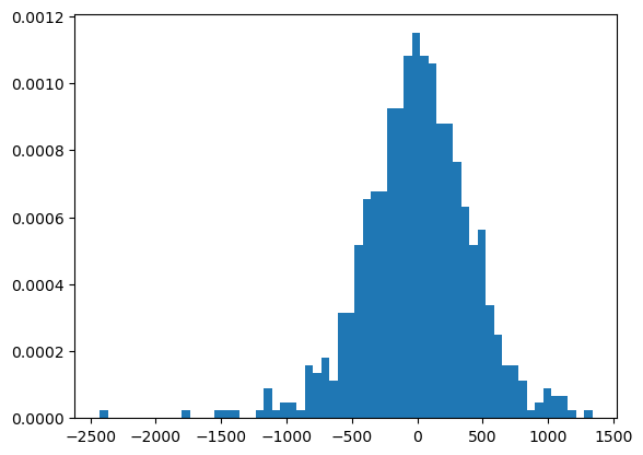
plt.figure()
plt.hist(dormir.fit().resid,bins = 60,density = True);
6.1.4. Transformaciones lineales#
uu = "https://raw.githubusercontent.com/vmoprojs/DataLectures/master/GA/Table%2031_3.csv"

datos = pd.read_csv(uu, sep =';')

reg_1 = stm.ols('Cellphone~Pcapincome',data = datos)
print(reg_1.fit().summary())
                            OLS Regression Results
==============================================================================
Dep. Variable:              Cellphone   R-squared:                       0.626
Model:                            OLS   Adj. R-squared:                  0.615
Method:                 Least Squares   F-statistic:                     53.67
Date:                Wed, 16 Apr 2025   Prob (F-statistic):           2.50e-08
Time:                        04:05:01   Log-Likelihood:                -148.94
No. Observations:                  34   AIC:                             301.9
Df Residuals:                      32   BIC:                             304.9
Df Model:                           1
Covariance Type:            nonrobust
==============================================================================
                 coef    std err          t      P>|t|      [0.025      0.975]
------------------------------------------------------------------------------
Intercept     12.4795      6.109      2.043      0.049       0.037      24.922
Pcapincome     0.0023      0.000      7.326      0.000       0.002       0.003
==============================================================================
Omnibus:                        1.398   Durbin-Watson:                   2.381
Prob(Omnibus):                  0.497   Jarque-Bera (JB):                0.531
Skew:                           0.225   Prob(JB):                        0.767
Kurtosis:                       3.414   Cond. No.                     3.46e+04
==============================================================================

Notes:
[1] Standard Errors assume that the covariance matrix of the errors is correctly specified.
[2] The condition number is large, 3.46e+04. This might indicate that there are
strong multicollinearity or other numerical problems.
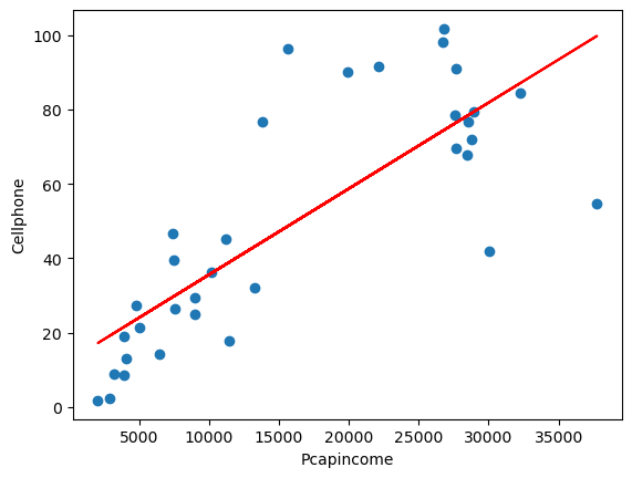
plt.figure()
plt.plot(datos.Pcapincome,datos.Cellphone,'o')
plt.plot(datos.Pcapincome,reg_1.fit().fittedvalues,'-',color='r')
plt.xlabel('Pcapincome')
plt.ylabel('Cellphone')
Text(0, 0.5, 'Cellphone')
6.1.5. Modelo reciproco#
uu =  "https://raw.githubusercontent.com/vmoprojs/DataLectures/master/GA/tabla_6_4.csv"
datos = pd.read_csv(uu,sep = ';')
datos.describe()
| CM | FLR | PGNP | TFR | |
|---|---|---|---|---|
| count | 64.000000 | 64.000000 | 64.000000 | 64.000000 |
| mean | 141.500000 | 51.187500 | 1401.250000 | 5.549688 |
| std | 75.978067 | 26.007859 | 2725.695775 | 1.508993 |
| min | 12.000000 | 9.000000 | 120.000000 | 1.690000 |
| 25% | 82.000000 | 29.000000 | 300.000000 | 4.607500 |
| 50% | 138.500000 | 48.000000 | 620.000000 | 6.040000 |
| 75% | 192.500000 | 77.250000 | 1317.500000 | 6.615000 |
| max | 312.000000 | 95.000000 | 19830.000000 | 8.490000 |
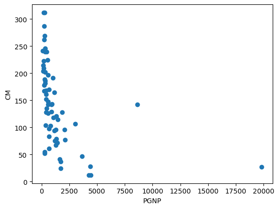
plt.figure()
plt.plot(datos.PGNP,datos.CM,'o')
plt.xlabel('PGNP')
plt.ylabel('CM')
Text(0, 0.5, 'CM')
reg1 = stm.ols('CM~PGNP',data = datos)
print(reg1.fit().summary())
                            OLS Regression Results
==============================================================================
Dep. Variable:                     CM   R-squared:                       0.166
Model:                            OLS   Adj. R-squared:                  0.153
Method:                 Least Squares   F-statistic:                     12.36
Date:                Wed, 16 Apr 2025   Prob (F-statistic):           0.000826
Time:                        04:05:02   Log-Likelihood:                -361.64
No. Observations:                  64   AIC:                             727.3
Df Residuals:                      62   BIC:                             731.6
Df Model:                           1
Covariance Type:            nonrobust
==============================================================================
                 coef    std err          t      P>|t|      [0.025      0.975]
------------------------------------------------------------------------------
Intercept    157.4244      9.846     15.989      0.000     137.743     177.105
PGNP          -0.0114      0.003     -3.516      0.001      -0.018      -0.005
==============================================================================
Omnibus:                        3.321   Durbin-Watson:                   1.931
Prob(Omnibus):                  0.190   Jarque-Bera (JB):                2.545
Skew:                           0.345   Prob(JB):                        0.280
Kurtosis:                       2.309   Cond. No.                     3.43e+03
==============================================================================

Notes:
[1] Standard Errors assume that the covariance matrix of the errors is correctly specified.
[2] The condition number is large, 3.43e+03. This might indicate that there are
strong multicollinearity or other numerical problems.
datos['RepPGNP'] = 1/datos.PGNP

reg2 = stm.ols('CM~RepPGNP',data = datos)
print(reg2.fit().summary())
                            OLS Regression Results
==============================================================================
Dep. Variable:                     CM   R-squared:                       0.459
Model:                            OLS   Adj. R-squared:                  0.450
Method:                 Least Squares   F-statistic:                     52.61
Date:                Wed, 16 Apr 2025   Prob (F-statistic):           7.82e-10
Time:                        04:05:02   Log-Likelihood:                -347.79
No. Observations:                  64   AIC:                             699.6
Df Residuals:                      62   BIC:                             703.9
Df Model:                           1
Covariance Type:            nonrobust
==============================================================================
                 coef    std err          t      P>|t|      [0.025      0.975]
------------------------------------------------------------------------------
Intercept     81.7944     10.832      7.551      0.000      60.141     103.447
RepPGNP     2.727e+04   3759.999      7.254      0.000    1.98e+04    3.48e+04
==============================================================================
Omnibus:                        0.147   Durbin-Watson:                   1.959
Prob(Omnibus):                  0.929   Jarque-Bera (JB):                0.334
Skew:                           0.065   Prob(JB):                        0.846
Kurtosis:                       2.671   Cond. No.                         534.
==============================================================================

Notes:
[1] Standard Errors assume that the covariance matrix of the errors is correctly specified.
6.1.6. Modelo log-lineal#
uu = "https://raw.githubusercontent.com/vmoprojs/DataLectures/master/WO/ceosal2.csv"

datos = pd.read_csv(uu,header = None)
datos.columns = ["salary", "age", "college", "grad", "comten", "ceoten", "sales", "profits","mktval", "lsalary", "lsales", "lmktval", "comtensq", "ceotensq", "profmarg"]
datos.head()


reg1 = stm.ols('lsalary~ceoten',data = datos)
print(reg1.fit().summary())
                            OLS Regression Results
==============================================================================
Dep. Variable:                lsalary   R-squared:                       0.013
Model:                            OLS   Adj. R-squared:                  0.008
Method:                 Least Squares   F-statistic:                     2.334
Date:                Wed, 16 Apr 2025   Prob (F-statistic):              0.128
Time:                        04:05:03   Log-Likelihood:                -160.84
No. Observations:                 177   AIC:                             325.7
Df Residuals:                     175   BIC:                             332.0
Df Model:                           1
Covariance Type:            nonrobust
==============================================================================
                 coef    std err          t      P>|t|      [0.025      0.975]
------------------------------------------------------------------------------
Intercept      6.5055      0.068     95.682      0.000       6.371       6.640
ceoten         0.0097      0.006      1.528      0.128      -0.003       0.022
==============================================================================
Omnibus:                        3.858   Durbin-Watson:                   2.084
Prob(Omnibus):                  0.145   Jarque-Bera (JB):                3.907
Skew:                          -0.189   Prob(JB):                        0.142
Kurtosis:                       3.622   Cond. No.                         16.1
==============================================================================

Notes:
[1] Standard Errors assume that the covariance matrix of the errors is correctly specified.
6.1.7. Regresión a través del origen#
uu = "https://raw.githubusercontent.com/vmoprojs/DataLectures/master/GA/Table%206_1.csv"
datos = pd.read_csv(uu,sep = ';')
datos.head()


lmod1 = stm.ols('Y~ -1+X',data = datos)
print(lmod1.fit().summary())
                                 OLS Regression Results
=======================================================================================
Dep. Variable:                      Y   R-squared (uncentered):                   0.502
Model:                            OLS   Adj. R-squared (uncentered):              0.500
Method:                 Least Squares   F-statistic:                              241.2
Date:                Wed, 16 Apr 2025   Prob (F-statistic):                    4.41e-38
Time:                        04:05:03   Log-Likelihood:                         -751.30
No. Observations:                 240   AIC:                                      1505.
Df Residuals:                     239   BIC:                                      1508.
Df Model:                           1
Covariance Type:            nonrobust
==============================================================================
                 coef    std err          t      P>|t|      [0.025      0.975]
------------------------------------------------------------------------------
X              1.1555      0.074     15.532      0.000       1.009       1.302
==============================================================================
Omnibus:                        9.576   Durbin-Watson:                   1.973
Prob(Omnibus):                  0.008   Jarque-Bera (JB):               13.569
Skew:                          -0.268   Prob(JB):                      0.00113
Kurtosis:                       4.034   Cond. No.                         1.00
==============================================================================

Notes:
[1] R² is computed without centering (uncentered) since the model does not contain a constant.
[2] Standard Errors assume that the covariance matrix of the errors is correctly specified.
6.2. Regresión Lineal Múltiple#
uu =  "https://raw.githubusercontent.com/vmoprojs/DataLectures/master/WO/hprice1.csv"
datos = pd.read_csv(uu,header=None)
datos.columns = ["price"   ,  "assess"  ,
                 "bdrms"  ,   "lotsize"  ,
                 "sqrft"   ,  "colonial",
                 "lprice"  ,  "lassess" ,
                 "llotsize" , "lsqrft"]

datos.describe()
| price | assess | bdrms | lotsize | sqrft | colonial | lprice | lassess | llotsize | lsqrft | |
|---|---|---|---|---|---|---|---|---|---|---|
| count | 88.000000 | 88.000000 | 88.000000 | 88.000000 | 88.000000 | 88.000000 | 88.000000 | 88.000000 | 88.000000 | 88.000000 |
| mean | 293.546034 | 315.736364 | 3.568182 | 9019.863636 | 2013.693182 | 0.693182 | 5.633180 | 5.717994 | 8.905105 | 7.572610 |
| std | 102.713445 | 95.314437 | 0.841393 | 10174.150414 | 577.191583 | 0.463816 | 0.303573 | 0.262113 | 0.544060 | 0.258688 |
| min | 111.000000 | 198.700000 | 2.000000 | 1000.000000 | 1171.000000 | 0.000000 | 4.709530 | 5.291796 | 6.907755 | 7.065613 |
| 25% | 230.000000 | 253.900000 | 3.000000 | 5732.750000 | 1660.500000 | 0.000000 | 5.438079 | 5.536940 | 8.653908 | 7.414873 |
| 50% | 265.500000 | 290.200000 | 3.000000 | 6430.000000 | 1845.000000 | 1.000000 | 5.581613 | 5.670566 | 8.768719 | 7.520231 |
| 75% | 326.250000 | 352.125000 | 4.000000 | 8583.250000 | 2227.000000 | 1.000000 | 5.787642 | 5.863982 | 9.057567 | 7.708266 |
| max | 725.000000 | 708.600000 | 7.000000 | 92681.000000 | 3880.000000 | 1.000000 | 6.586172 | 6.563291 | 11.436920 | 8.263591 |
modelo1 = stm.ols('lprice~lassess+llotsize+lsqrft+bdrms',data = datos)
print(modelo1.fit().summary())
                            OLS Regression Results
==============================================================================
Dep. Variable:                 lprice   R-squared:                       0.773
Model:                            OLS   Adj. R-squared:                  0.762
Method:                 Least Squares   F-statistic:                     70.58
Date:                Wed, 16 Apr 2025   Prob (F-statistic):           6.45e-26
Time:                        04:05:04   Log-Likelihood:                 45.750
No. Observations:                  88   AIC:                            -81.50
Df Residuals:                      83   BIC:                            -69.11
Df Model:                           4
Covariance Type:            nonrobust
==============================================================================
                 coef    std err          t      P>|t|      [0.025      0.975]
------------------------------------------------------------------------------
Intercept      0.2637      0.570      0.463      0.645      -0.869       1.397
lassess        1.0431      0.151      6.887      0.000       0.742       1.344
llotsize       0.0074      0.039      0.193      0.848      -0.069       0.084
lsqrft        -0.1032      0.138     -0.746      0.458      -0.379       0.172
bdrms          0.0338      0.022      1.531      0.129      -0.010       0.078
==============================================================================
Omnibus:                       14.527   Durbin-Watson:                   2.048
Prob(Omnibus):                  0.001   Jarque-Bera (JB):               56.436
Skew:                           0.118   Prob(JB):                     5.56e-13
Kurtosis:                       6.916   Cond. No.                         501.
==============================================================================

Notes:
[1] Standard Errors assume that the covariance matrix of the errors is correctly specified.
modelo2 = stm.ols('lprice~llotsize+lsqrft+bdrms',data = datos)
print(modelo2.fit().summary())
                            OLS Regression Results
==============================================================================
Dep. Variable:                 lprice   R-squared:                       0.643
Model:                            OLS   Adj. R-squared:                  0.630
Method:                 Least Squares   F-statistic:                     50.42
Date:                Wed, 16 Apr 2025   Prob (F-statistic):           9.74e-19
Time:                        04:05:04   Log-Likelihood:                 25.861
No. Observations:                  88   AIC:                            -43.72
Df Residuals:                      84   BIC:                            -33.81
Df Model:                           3
Covariance Type:            nonrobust
==============================================================================
                 coef    std err          t      P>|t|      [0.025      0.975]
------------------------------------------------------------------------------
Intercept     -1.2970      0.651     -1.992      0.050      -2.592      -0.002
llotsize       0.1680      0.038      4.388      0.000       0.092       0.244
lsqrft         0.7002      0.093      7.540      0.000       0.516       0.885
bdrms          0.0370      0.028      1.342      0.183      -0.018       0.092
==============================================================================
Omnibus:                       12.060   Durbin-Watson:                   2.089
Prob(Omnibus):                  0.002   Jarque-Bera (JB):               34.890
Skew:                          -0.188   Prob(JB):                     2.65e-08
Kurtosis:                       6.062   Cond. No.                         410.
==============================================================================

Notes:
[1] Standard Errors assume that the covariance matrix of the errors is correctly specified.
modelo3 = stm.ols('lprice~bdrms',data = datos)
print(modelo3.fit().summary())
                            OLS Regression Results
==============================================================================
Dep. Variable:                 lprice   R-squared:                       0.215
Model:                            OLS   Adj. R-squared:                  0.206
Method:                 Least Squares   F-statistic:                     23.53
Date:                Wed, 16 Apr 2025   Prob (F-statistic):           5.43e-06
Time:                        04:05:04   Log-Likelihood:                -8.8147
No. Observations:                  88   AIC:                             21.63
Df Residuals:                      86   BIC:                             26.58
Df Model:                           1
Covariance Type:            nonrobust
==============================================================================
                 coef    std err          t      P>|t|      [0.025      0.975]
------------------------------------------------------------------------------
Intercept      5.0365      0.126     39.862      0.000       4.785       5.288
bdrms          0.1672      0.034      4.851      0.000       0.099       0.236
==============================================================================
Omnibus:                        7.476   Durbin-Watson:                   2.056
Prob(Omnibus):                  0.024   Jarque-Bera (JB):               13.085
Skew:                          -0.182   Prob(JB):                      0.00144
Kurtosis:                       4.854   Cond. No.                         17.2
==============================================================================

Notes:
[1] Standard Errors assume that the covariance matrix of the errors is correctly specified.
import seaborn as sns

sns.pairplot(datos.loc[:,['lprice','llotsize' , 'lsqrft' , 'bdrms']])
<seaborn.axisgrid.PairGrid at 0x7fc180367df0>

6.2.1. Predicción#
datos_nuevos = pd.DataFrame({'llotsize':np.log(2100),'lsqrft':np.log(8000),'bdrms':4},index = [0])

pred_vals = modelo2.fit().predict()
modelo2.fit().get_prediction().summary_frame().head()
| mean | mean_se | mean_ci_lower | mean_ci_upper | obs_ci_lower | obs_ci_upper | |
|---|---|---|---|---|---|---|
| 0 | 5.776577 | 0.029185 | 5.718541 | 5.834614 | 5.404916 | 6.148239 |
| 1 | 5.707740 | 0.029306 | 5.649463 | 5.766018 | 5.336041 | 6.079440 |
| 2 | 5.310543 | 0.033384 | 5.244156 | 5.376930 | 4.937486 | 5.683600 |
| 3 | 5.326681 | 0.031818 | 5.263407 | 5.389955 | 4.954165 | 5.699197 |
| 4 | 5.797220 | 0.031014 | 5.735544 | 5.858895 | 5.424972 | 6.169467 |
pred_vals = modelo2.fit().get_prediction(datos_nuevos)
pred_vals.summary_frame()
| mean | mean_se | mean_ci_lower | mean_ci_upper | obs_ci_lower | obs_ci_upper | |
|---|---|---|---|---|---|---|
| 0 | 6.428811 | 0.147975 | 6.134546 | 6.723076 | 5.958326 | 6.899296 |
6.2.2. RLM: Cobb-Douglas#
El modelo:
donde
\(Y\): producción
\(X_2\): insumo trabajo
\(X_3\): insumo capital
\(u\): término de perturbación
\(e\): base del logaritmo
Notemos que el modelo es multiplicativo, si tomamos la derivada obetenemos un modelo más famliar respecto a la regresión lineal múltiple:
La interpretación de los coeficientes es []:
\(\beta_2\) es la elasticidad (parcial) de la producción respecto del insumo trabajo, es decir, mide el cambio porcentual en la producción debido a una variación de 1% en el insumo trabajo, con el insumo capital constante.
De igual forma, \(\beta_3\) es la elasticidad (parcial) de la producción respecto del insumo capital, con el insumo trabajo constante.
La suma (\(\beta_2+\beta_3\)) da información sobre los rendimientos a escala, es decir, la respuesta de la producción a un cambio proporcional en los insumos. Si esta suma es 1, existen rendimientos constantes a escala, es decir, la duplicación de los insumos duplica la producción, la triplicación de los insumos la triplica, y así sucesivamente. Si la suma es menor que 1, existen rendimientos decrecientes a escala: al duplicar los insumos, la producción crece en menos del doble. Por último, si la suma es mayor que 1, hay rendimientos crecientes a escala; la duplicación de los insumos aumenta la producción en más del doble.
Abrir la tabla 7.3. Regresar las horas de trabajo (\(X_2\)) e Inversión de Capital (\(X_3\)) en el Valor Agregado (\(Y\))
uu = "https://raw.githubusercontent.com/vmoprojs/DataLectures/master/GA/tabla7_3.csv"
datos =  pd.read_csv(uu,sep=";")
datos.describe()
| Year | Y | X2 | X3 | |
|---|---|---|---|---|
| count | 15.000000 | 15.000000 | 15.000000 | 15.000000 |
| mean | 1965.000000 | 24735.333333 | 287.346667 | 25505.966667 |
| std | 4.472136 | 4874.173486 | 14.806556 | 7334.889966 |
| min | 1958.000000 | 16607.700000 | 267.000000 | 17803.700000 |
| 25% | 1961.500000 | 20618.800000 | 274.700000 | 19407.450000 |
| 50% | 1965.000000 | 26465.800000 | 288.100000 | 23445.200000 |
| 75% | 1968.500000 | 28832.100000 | 299.850000 | 30766.850000 |
| max | 1972.000000 | 31535.800000 | 307.500000 | 41794.300000 |
W = np.log(datos.X2)

K = np.log(datos.X3)

LY = np.log(datos.Y)

reg_1 = stm.ols("LY~W+K",data = datos).fit()
print(reg_1.summary())
import statsmodels.api as sm
sm.stats.anova_lm(reg_1, typ=2)
/Users/victormorales/opt/anaconda3/lib/python3.9/site-packages/scipy/stats/_stats_py.py:1806: UserWarning: kurtosistest only valid for n>=20 ... continuing anyway, n=15
  warnings.warn("kurtosistest only valid for n>=20 ... continuing "
                            OLS Regression Results
==============================================================================
Dep. Variable:                     LY   R-squared:                       0.889
Model:                            OLS   Adj. R-squared:                  0.871
Method:                 Least Squares   F-statistic:                     48.08
Date:                Wed, 16 Apr 2025   Prob (F-statistic):           1.86e-06
Time:                        04:05:08   Log-Likelihood:                 19.284
No. Observations:                  15   AIC:                            -32.57
Df Residuals:                      12   BIC:                            -30.44
Df Model:                           2
Covariance Type:            nonrobust
==============================================================================
                 coef    std err          t      P>|t|      [0.025      0.975]
------------------------------------------------------------------------------
Intercept     -3.3387      2.449     -1.363      0.198      -8.675       1.998
W              1.4987      0.540      2.777      0.017       0.323       2.675
K              0.4899      0.102      4.801      0.000       0.268       0.712
==============================================================================
Omnibus:                        3.290   Durbin-Watson:                   0.891
Prob(Omnibus):                  0.193   Jarque-Bera (JB):                1.723
Skew:                          -0.827   Prob(JB):                        0.422
Kurtosis:                       3.141   Cond. No.                     1.51e+03
==============================================================================

Notes:
[1] Standard Errors assume that the covariance matrix of the errors is correctly specified.
[2] The condition number is large, 1.51e+03. This might indicate that there are
strong multicollinearity or other numerical problems.
| sum_sq | df | F | PR(>F) | |
|---|---|---|---|---|
| W | 0.043141 | 1.0 | 7.710533 | 0.016750 |
| K | 0.128988 | 1.0 | 23.053747 | 0.000432 |
| Residual | 0.067141 | 12.0 | NaN | NaN |
Las elasticidades de la producción respecto del trabajo y el capital fueron 1.49 y 0.48 respectivamente.
Ahora, si existen rendimientos constantes a escala (un cambio equi-proporcional en la producción ante un cambio equi-proporcional en los insumos), la teoría económica sugeriría que:
LY_K = np.log(datos.Y/datos.X3)
W_K = np.log(datos.X2/datos.X3)


reg_2 = stm.ols("LY_K~W_K",data = datos).fit()
print(reg_2.summary())
sm.stats.anova_lm(reg_2)
                            OLS Regression Results
==============================================================================
Dep. Variable:                   LY_K   R-squared:                       0.570
Model:                            OLS   Adj. R-squared:                  0.536
Method:                 Least Squares   F-statistic:                     17.20
Date:                Wed, 16 Apr 2025   Prob (F-statistic):            0.00115
Time:                        04:05:09   Log-Likelihood:                 16.965
No. Observations:                  15   AIC:                            -29.93
Df Residuals:                      13   BIC:                            -28.51
Df Model:                           1
Covariance Type:            nonrobust
==============================================================================
                 coef    std err          t      P>|t|      [0.025      0.975]
------------------------------------------------------------------------------
Intercept      1.7083      0.416      4.108      0.001       0.810       2.607
W_K            0.3870      0.093      4.147      0.001       0.185       0.589
==============================================================================
Omnibus:                        0.801   Durbin-Watson:                   0.601
Prob(Omnibus):                  0.670   Jarque-Bera (JB):                0.749
Skew:                          -0.431   Prob(JB):                        0.688
Kurtosis:                       2.325   Cond. No.                         89.9
==============================================================================

Notes:
[1] Standard Errors assume that the covariance matrix of the errors is correctly specified.
/Users/victormorales/opt/anaconda3/lib/python3.9/site-packages/scipy/stats/_stats_py.py:1806: UserWarning: kurtosistest only valid for n>=20 ... continuing anyway, n=15
  warnings.warn("kurtosistest only valid for n>=20 ... continuing "
| df | sum_sq | mean_sq | F | PR(>F) | |
|---|---|---|---|---|---|
| W_K | 1.0 | 0.121005 | 0.121005 | 17.19981 | 0.001147 |
| Residual | 13.0 | 0.091459 | 0.007035 | NaN | NaN |
¿Se cumple la hipótesis nula? ¿Existen rendimientos constantes de escala?
Una forma de responder a la pregunta es mediante la prueba \(t\), para \(Ho: \beta_2 +\beta_3 = 1\), tenemos
donde la información nececesaria para obtener \(cov(\hat{\beta}_2,\hat{\beta}_3)\) en Python la librería statsmodels.api es model.cov_params() y model es el ajuste del modelo.
Otra forma de hacer la prueba es mediante el estadístico \(F\):
donde \(m\) es el número de restricciones lineales y \(k\) es el número de parámetros de la regresión no restringida.
SCRNR = 0.0671410
SCRRes = 0.09145854
numero_rest = 1
grad = 12

est_F = ((SCRRes-SCRNR)/numero_rest)/(SCRNR/grad)
est_F

from scipy import stats
mif = stats.f.cdf(est_F,dfn=1, dfd=12)
valorp = 1-mif
print(["Estadistico F: "] +[est_F])
print(["Valor p: "] +[valorp])
#cov_matrix = reg_1.cov_params()
#print(cov_matrix)
['Estadistico F: ', 4.346233746890871]
['Valor p: ', 0.059121842231030675]
No se tiene suficiente evidencia para rechazar la hipótesis nula de que sea una economía de escala.
Notemos que existe una relación directa entre el coeficiente de determinación o bondad de ajuste \(R^2\) y \(F\). En primero lugar, recordemos la descomposición de los errores:
De cuyos elementos podemos obtener tanto \(R^2\) como \(F\):
donde \(k\) es el número de variables (incluido el intercepto) y sigue una distribución \(F\) con \(k-1\) y \(n-k\) grados de libertad.
6.2.3. RLM: Dicotómicas#
Abrir los datos wage1 Correr los modelos. Se desea saber si el género tiene relación con el salario y en qué medida.
uu = "https://raw.githubusercontent.com/vmoprojs/DataLectures/master/WO/wage1.csv"
salarios = pd.read_csv(uu, header = None)

salarios.columns =  ["wage", "educ", "exper", "tenure", "nonwhite", "female", "married",
                     "numdep", "smsa", "northcen", "south", "west", "construc", "ndurman",
                     "trcommpu", "trade", "services",  "profserv", "profocc", "clerocc",
                     "servocc", "lwage", "expersq", "tenursq"]
reg3 = stm.ols("wage~female",data = salarios).fit()
print(reg3.summary())

reg4 = stm.ols("wage~female + educ+ exper + tenure",data = salarios).fit()
print(reg4.summary())
                            OLS Regression Results
==============================================================================
Dep. Variable:                   wage   R-squared:                       0.116
Model:                            OLS   Adj. R-squared:                  0.114
Method:                 Least Squares   F-statistic:                     68.54
Date:                Wed, 16 Apr 2025   Prob (F-statistic):           1.04e-15
Time:                        04:05:09   Log-Likelihood:                -1400.7
No. Observations:                 526   AIC:                             2805.
Df Residuals:                     524   BIC:                             2814.
Df Model:                           1
Covariance Type:            nonrobust
==============================================================================
                 coef    std err          t      P>|t|      [0.025      0.975]
------------------------------------------------------------------------------
Intercept      7.0995      0.210     33.806      0.000       6.687       7.512
female        -2.5118      0.303     -8.279      0.000      -3.108      -1.916
==============================================================================
Omnibus:                      223.488   Durbin-Watson:                   1.818
Prob(Omnibus):                  0.000   Jarque-Bera (JB):              929.998
Skew:                           1.928   Prob(JB):                    1.13e-202
Kurtosis:                       8.250   Cond. No.                         2.57
==============================================================================

Notes:
[1] Standard Errors assume that the covariance matrix of the errors is correctly specified.
                            OLS Regression Results
==============================================================================
Dep. Variable:                   wage   R-squared:                       0.364
Model:                            OLS   Adj. R-squared:                  0.359
Method:                 Least Squares   F-statistic:                     74.40
Date:                Wed, 16 Apr 2025   Prob (F-statistic):           7.30e-50
Time:                        04:05:09   Log-Likelihood:                -1314.2
No. Observations:                 526   AIC:                             2638.
Df Residuals:                     521   BIC:                             2660.
Df Model:                           4
Covariance Type:            nonrobust
==============================================================================
                 coef    std err          t      P>|t|      [0.025      0.975]
------------------------------------------------------------------------------
Intercept     -1.5679      0.725     -2.164      0.031      -2.991      -0.145
female        -1.8109      0.265     -6.838      0.000      -2.331      -1.291
educ           0.5715      0.049     11.584      0.000       0.475       0.668
exper          0.0254      0.012      2.195      0.029       0.003       0.048
tenure         0.1410      0.021      6.663      0.000       0.099       0.183
==============================================================================
Omnibus:                      185.864   Durbin-Watson:                   1.794
Prob(Omnibus):                  0.000   Jarque-Bera (JB):              715.580
Skew:                           1.589   Prob(JB):                    4.11e-156
Kurtosis:                       7.749   Cond. No.                         141.
==============================================================================

Notes:
[1] Standard Errors assume that the covariance matrix of the errors is correctly specified.
La hipótesis es saber si el coeficiente de female es menor a cero.
Se nota que es menor.
Tomando en cuenta, educacion experiencia y edad, en promedio a la mujer le pagan 1.81 menos
6.2.4. RLM: Educación con insumos#
Abrir los datos gpa1 Correr los modelos.
¿Afecta el promedio de calificaciones el tener o no una computadora?
uu = "https://raw.githubusercontent.com/vmoprojs/DataLectures/master/WO/gpa1.csv"
datosgpa = pd.read_csv(uu, header = None)
datosgpa.columns = ["age",  "soph",  "junior",    "senior",    "senior5",  "male", "campus",   "business", "engineer", "colGPA",   "hsGPA",    "ACT",  "job19",    "job20",    "drive",    "bike", "walk", "voluntr",  "PC",   "greek",    "car",  "siblings", "bgfriend", "clubs",    "skipped",  "alcohol",  "gradMI",   "fathcoll", "mothcoll"]

reg4 = stm.ols('colGPA ~ PC', data = datosgpa)
print(reg4.fit().summary())
                            OLS Regression Results
==============================================================================
Dep. Variable:                 colGPA   R-squared:                       0.050
Model:                            OLS   Adj. R-squared:                  0.043
Method:                 Least Squares   F-statistic:                     7.314
Date:                Wed, 16 Apr 2025   Prob (F-statistic):            0.00770
Time:                        04:05:10   Log-Likelihood:                -56.641
No. Observations:                 141   AIC:                             117.3
Df Residuals:                     139   BIC:                             123.2
Df Model:                           1
Covariance Type:            nonrobust
==============================================================================
                 coef    std err          t      P>|t|      [0.025      0.975]
------------------------------------------------------------------------------
Intercept      2.9894      0.040     75.678      0.000       2.911       3.068
PC             0.1695      0.063      2.704      0.008       0.046       0.293
==============================================================================
Omnibus:                        2.136   Durbin-Watson:                   1.941
Prob(Omnibus):                  0.344   Jarque-Bera (JB):                1.852
Skew:                           0.160   Prob(JB):                        0.396
Kurtosis:                       2.539   Cond. No.                         2.45
==============================================================================

Notes:
[1] Standard Errors assume that the covariance matrix of the errors is correctly specified.
reg5 = stm.ols('colGPA ~ PC + hsGPA + ACT', data = datosgpa)
print(reg5.fit().summary())
                            OLS Regression Results
==============================================================================
Dep. Variable:                 colGPA   R-squared:                       0.219
Model:                            OLS   Adj. R-squared:                  0.202
Method:                 Least Squares   F-statistic:                     12.83
Date:                Wed, 16 Apr 2025   Prob (F-statistic):           1.93e-07
Time:                        04:05:10   Log-Likelihood:                -42.796
No. Observations:                 141   AIC:                             93.59
Df Residuals:                     137   BIC:                             105.4
Df Model:                           3
Covariance Type:            nonrobust
==============================================================================
                 coef    std err          t      P>|t|      [0.025      0.975]
------------------------------------------------------------------------------
Intercept      1.2635      0.333      3.793      0.000       0.605       1.922
PC             0.1573      0.057      2.746      0.007       0.044       0.271
hsGPA          0.4472      0.094      4.776      0.000       0.262       0.632
ACT            0.0087      0.011      0.822      0.413      -0.012       0.029
==============================================================================
Omnibus:                        2.770   Durbin-Watson:                   1.870
Prob(Omnibus):                  0.250   Jarque-Bera (JB):                1.863
Skew:                           0.016   Prob(JB):                        0.394
Kurtosis:                       2.438   Cond. No.                         298.
==============================================================================

Notes:
[1] Standard Errors assume that the covariance matrix of the errors is correctly specified.
6.2.5. RLM: Cambio estructural#
Cuando utilizamos un modelo de regresión que implica series de tiempo, tal vez se dé un cambio estructural en la relación entre la regresada Y y las regresoras. Por cambio estructural nos referimos a que los valores de los parámetros del modelo no permanecen constantes a lo largo de todo el periodo []
Se sabe muy bien que en 1982 Estados Unidos experimentó su peor recesión en tiempos de paz. La tasa de desempleo civil alcanzó 9.7%, la más alta desde 1948. Un suceso como éste pudo perturbar la relación entre el ahorro y el IPD. Para ver si lo anterior sucedió, dividamos la muestra en dos periodos: 1970-1981 y 1982-1995, antes y después de la recesión de 1982.
Ahora tenemos tres posibles regresiones:
De los períodos parciales se desprende cuatro posibilidades:
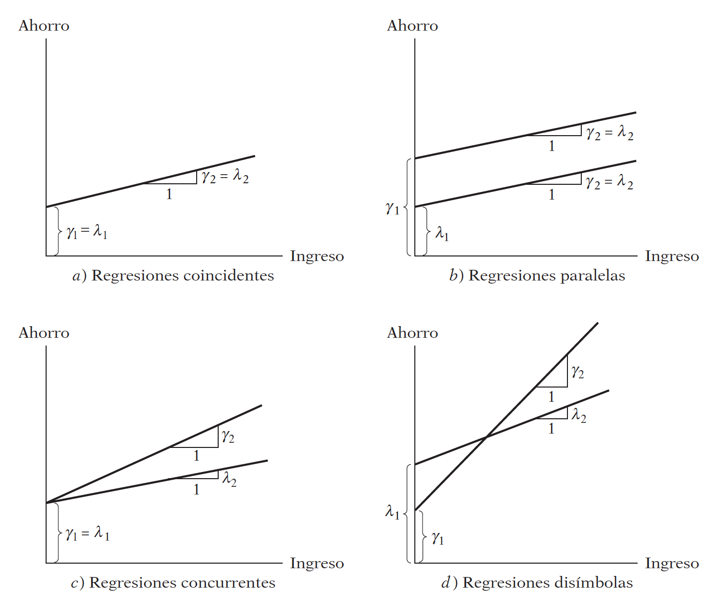
Para evaluar si hay diferencias, podemos utilizar los modelos de regresión con variables dicotómicas:
donde
\(Y\): ahorro
\(X\): ingreso
\(t\): tiempo
\(D\): 1 para el período 1982-1995, 0 en otro caso.
La variable dicotómica de la ecuación (6.3) es quien me permite estimar las ecuaciones (6.1) y (6.2) al mismo tiempo. Es decir:
Función de ahorros medios para 1970-1981:
Función de ahorros medios para 1982-1995:
Notemos que se trata de las mismas funciones que en (6.1) y (6.2), con
\(\lambda_1=\alpha_1\)
\(\lambda_2=\beta_1\)
\(\gamma_1=(\alpha_1+\alpha_2)\)
\(\gamma_2=(\beta_1+\beta_2)\)
Abrir los datos 8.9. Veamos las variables gráficamente:
uu = "https://raw.githubusercontent.com/vmoprojs/DataLectures/master/GA/tabla_8_9.csv"

datos = pd.read_csv(uu,sep=";")
datos.columns
Index(['YEAR', 'SAVINGS', 'INCOME'], dtype='object')
import matplotlib.pyplot as plt
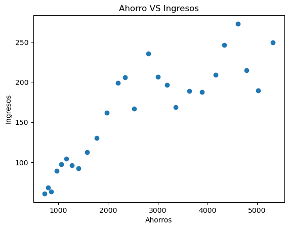
plt.scatter(datos.INCOME,datos.SAVINGS)
plt.gca().update(dict(title='Ahorro VS Ingresos', xlabel='Ahorros', ylabel='Ingresos'))
[Text(0.5, 1.0, 'Ahorro VS Ingresos'),
 Text(0.5, 0, 'Ahorros'),
 Text(0, 0.5, 'Ingresos')]
plt.plot(datos.YEAR,datos.SAVINGS,"--o")
plt.gca().update(dict(title='Ahorro VS Tiempo', xlabel='Año', ylabel='Ahorro'))
[Text(0.5, 1.0, 'Ahorro VS Tiempo'),
 Text(0.5, 0, 'Año'),
 Text(0, 0.5, 'Ahorro')]
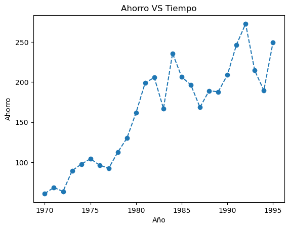
¿Hubo algún cambio en la relación entre ingreso y ahorro en el 80?
Hay varias formas de hacer la prueba, la mas fácil es mediante variables dicotómicas
ajuste_chow = stm.ols("SAVINGS~INCOME",data = datos).fit()
print(ajuste_chow.summary())

cambio = (datos.YEAR>1981)*1

ajuste_chow = stm.ols("SAVINGS~INCOME+cambio",data = datos).fit()
print(ajuste_chow.summary())
                            OLS Regression Results
==============================================================================
Dep. Variable:                SAVINGS   R-squared:                       0.767
Model:                            OLS   Adj. R-squared:                  0.758
Method:                 Least Squares   F-statistic:                     79.10
Date:                Wed, 16 Apr 2025   Prob (F-statistic):           4.61e-09
Time:                        04:05:10   Log-Likelihood:                -125.24
No. Observations:                  26   AIC:                             254.5
Df Residuals:                      24   BIC:                             257.0
Df Model:                           1
Covariance Type:            nonrobust
==============================================================================
                 coef    std err          t      P>|t|      [0.025      0.975]
------------------------------------------------------------------------------
Intercept     62.4227     12.761      4.892      0.000      36.086      88.760
INCOME         0.0377      0.004      8.894      0.000       0.029       0.046
==============================================================================
Omnibus:                        1.662   Durbin-Watson:                   0.860
Prob(Omnibus):                  0.436   Jarque-Bera (JB):                1.171
Skew:                           0.515   Prob(JB):                        0.557
Kurtosis:                       2.863   Cond. No.                     6.30e+03
==============================================================================

Notes:
[1] Standard Errors assume that the covariance matrix of the errors is correctly specified.
[2] The condition number is large, 6.3e+03. This might indicate that there are
strong multicollinearity or other numerical problems.
                            OLS Regression Results
==============================================================================
Dep. Variable:                SAVINGS   R-squared:                       0.792
Model:                            OLS   Adj. R-squared:                  0.774
Method:                 Least Squares   F-statistic:                     43.76
Date:                Wed, 16 Apr 2025   Prob (F-statistic):           1.45e-08
Time:                        04:05:10   Log-Likelihood:                -123.78
No. Observations:                  26   AIC:                             253.6
Df Residuals:                      23   BIC:                             257.3
Df Model:                           2
Covariance Type:            nonrobust
==============================================================================
                 coef    std err          t      P>|t|      [0.025      0.975]
------------------------------------------------------------------------------
Intercept     71.7059     13.546      5.294      0.000      43.685      99.727
INCOME         0.0265      0.008      3.340      0.003       0.010       0.043
cambio        37.8335     22.905      1.652      0.112      -9.549      85.216
==============================================================================
Omnibus:                        2.327   Durbin-Watson:                   1.046
Prob(Omnibus):                  0.312   Jarque-Bera (JB):                1.671
Skew:                           0.619   Prob(JB):                        0.434
Kurtosis:                       2.899   Cond. No.                     1.22e+04
==============================================================================

Notes:
[1] Standard Errors assume that the covariance matrix of the errors is correctly specified.
[2] The condition number is large, 1.22e+04. This might indicate that there are
strong multicollinearity or other numerical problems.
Veamos el modelo en términos de interacciones y la matriz de diseño:
ajuste_chow1 = stm.ols("SAVINGS~INCOME+cambio+INCOME*cambio", data = datos).fit()
print(ajuste_chow1.summary())
                            OLS Regression Results
==============================================================================
Dep. Variable:                SAVINGS   R-squared:                       0.882
Model:                            OLS   Adj. R-squared:                  0.866
Method:                 Least Squares   F-statistic:                     54.78
Date:                Wed, 16 Apr 2025   Prob (F-statistic):           2.27e-10
Time:                        04:05:10   Log-Likelihood:                -116.41
No. Observations:                  26   AIC:                             240.8
Df Residuals:                      22   BIC:                             245.9
Df Model:                           3
Covariance Type:            nonrobust
=================================================================================
                    coef    std err          t      P>|t|      [0.025      0.975]
---------------------------------------------------------------------------------
Intercept         1.0161     20.165      0.050      0.960     -40.803      42.835
INCOME            0.0803      0.014      5.541      0.000       0.050       0.110
cambio          152.4786     33.082      4.609      0.000      83.870     221.087
INCOME:cambio    -0.0655      0.016     -4.096      0.000      -0.099      -0.032
==============================================================================
Omnibus:                        0.861   Durbin-Watson:                   1.648
Prob(Omnibus):                  0.650   Jarque-Bera (JB):                0.596
Skew:                           0.360   Prob(JB):                        0.742
Kurtosis:                       2.822   Cond. No.                     3.24e+04
==============================================================================

Notes:
[1] Standard Errors assume that the covariance matrix of the errors is correctly specified.
[2] The condition number is large, 3.24e+04. This might indicate that there are
strong multicollinearity or other numerical problems.
6.3. RLM: Supuestos#
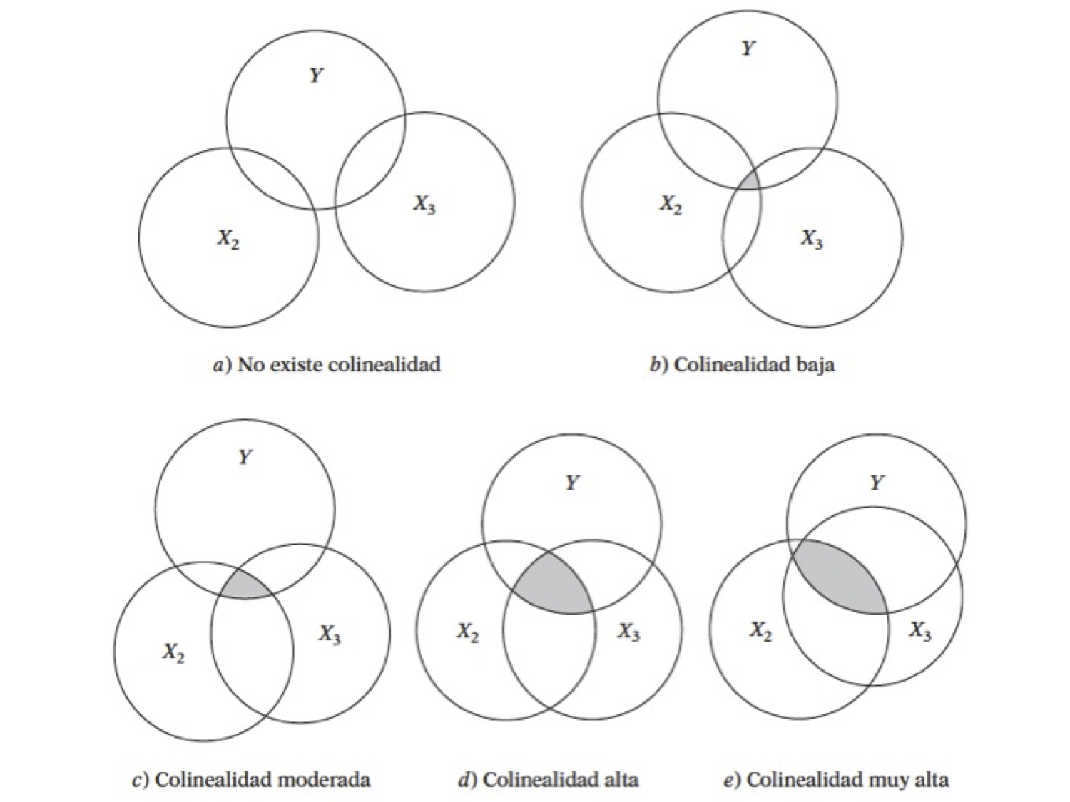
6.3.1. Multicolinealidad#
El problema:
Se tiene un problema en cuanto a la transpuesta de la matriz \((X'X)\)
Perfecta: Si se tiene este tipo, el modelo simplemente no toma en cuenta esta variable
Imperfecta: El cáclulo de la inversa es computacionalmente exigente
Posibles causas:
El método de recolección de información
Restricciones en el modelo o en la población objeto de muestreo
Especificación del modelo
Un modelo sobredetermindado
Series de tiempo
¿Cuál es la naturaleza de la multicolinealidad?
Causas
¿Cuáles son sus consecuencias prácticas?
Incidencia en los errores estándar y sensibilidad
¿Cómo se detecta?
Pruebas
¿Qué medidas pueden tomarse para aliviar el problema de multicolinealidad?
No hacer nada
Eliminar variables
Transformación de variables
Añadir datos a la muestra
Componentes principales, factores, entre otros
¿Cómo se detecta?
Un \(R^{2}\) elevado pero con pocas razones \(t\) significativas
Regresiones auxiliares (Pruebas de Klein)
Factor de inflación de la varianza
Ejemplo 1
Haremos uso del paquete AER
Abrir la tabla 10.8
Ajusta el modelo
donde
\(X_1\) índice implícito de deflación de precios para el PIB,
\(X_2\) es el PIB (en millones de dólares),
\(X_3\) número de desempleados (en miles),
\(X_4\) número de personas enlistadas en las fuerzas armadas,
\(X_5\) población no institucionalizada mayor de 14 años de edad
\(X_6\) año (igual a 1 para 1947, 2 para 1948 y 16 para 1962).
Analice los resultados
uu = "https://raw.githubusercontent.com/vmoprojs/DataLectures/master/GA/tabla10_8.csv"
datos =  pd.read_csv(uu,sep = ";")
datos.describe()
| obs | Y | X1 | X2 | X3 | X4 | X5 | TIME | |
|---|---|---|---|---|---|---|---|---|
| count | 15.000000 | 15.000000 | 15.000000 | 15.000000 | 15.000000 | 15.000000 | 15.000000 | 15.000000 |
| mean | 1954.000000 | 64968.066667 | 1006.666667 | 376552.066667 | 3139.066667 | 2592.000000 | 116580.200000 | 8.000000 |
| std | 4.472136 | 3335.820235 | 103.503393 | 91951.976996 | 940.825053 | 717.773741 | 6295.863769 | 4.472136 |
| min | 1947.000000 | 60171.000000 | 830.000000 | 234289.000000 | 1870.000000 | 1456.000000 | 107608.000000 | 1.000000 |
| 25% | 1950.500000 | 62204.000000 | 928.500000 | 306787.000000 | 2340.500000 | 2082.000000 | 111502.000000 | 4.500000 |
| 50% | 1954.000000 | 64989.000000 | 1000.000000 | 365385.000000 | 2936.000000 | 2637.000000 | 116219.000000 | 8.000000 |
| 75% | 1957.500000 | 68013.000000 | 1096.000000 | 443657.500000 | 3747.500000 | 3073.500000 | 121197.500000 | 11.500000 |
| max | 1961.000000 | 69564.000000 | 1157.000000 | 518173.000000 | 4806.000000 | 3594.000000 | 127852.000000 | 15.000000 |
Agreguemos el tiempo:
Las correlaciones muy altas también suelen ser síntoma de multicolinealidad
ajuste2 = stm.ols("Y~X1+X2+X3+X4+X5+TIME",data = datos).fit()
print(ajuste2.summary())
                            OLS Regression Results
==============================================================================
Dep. Variable:                      Y   R-squared:                       0.996
Model:                            OLS   Adj. R-squared:                  0.992
Method:                 Least Squares   F-statistic:                     295.8
Date:                Wed, 16 Apr 2025   Prob (F-statistic):           6.04e-09
Time:                        04:05:11   Log-Likelihood:                -101.91
No. Observations:                  15   AIC:                             217.8
Df Residuals:                       8   BIC:                             222.8
Df Model:                           6
Covariance Type:            nonrobust
==============================================================================
                 coef    std err          t      P>|t|      [0.025      0.975]
------------------------------------------------------------------------------
Intercept   6.727e+04   2.32e+04      2.895      0.020    1.37e+04    1.21e+05
X1            -2.0511      8.710     -0.235      0.820     -22.136      18.034
X2            -0.0273      0.033     -0.824      0.434      -0.104       0.049
X3            -1.9523      0.477     -4.095      0.003      -3.052      -0.853
X4            -0.9582      0.216     -4.432      0.002      -1.457      -0.460
X5             0.0513      0.234      0.219      0.832      -0.488       0.591
TIME        1585.1555    482.683      3.284      0.011     472.086    2698.225
==============================================================================
Omnibus:                        1.044   Durbin-Watson:                   2.492
Prob(Omnibus):                  0.593   Jarque-Bera (JB):                0.418
Skew:                           0.408   Prob(JB):                        0.811
Kurtosis:                       2.929   Cond. No.                     1.23e+08
==============================================================================

Notes:
[1] Standard Errors assume that the covariance matrix of the errors is correctly specified.
[2] The condition number is large, 1.23e+08. This might indicate that there are
strong multicollinearity or other numerical problems.
/Users/victormorales/opt/anaconda3/lib/python3.9/site-packages/scipy/stats/_stats_py.py:1806: UserWarning: kurtosistest only valid for n>=20 ... continuing anyway, n=15
  warnings.warn("kurtosistest only valid for n>=20 ... continuing "
X = datos[['X1','X2','X3','X4','X5','TIME']]
np.corrcoef(X)
array([[1.        , 0.99924002, 0.99943568, 0.99769462, 0.99320207,
        0.99142138, 0.98987707, 0.99050446, 0.98686967, 0.98485669,
        0.98283221, 0.98314407, 0.97959391, 0.97833135, 0.97770034],
       [0.99924002, 1.        , 0.9999722 , 0.99957845, 0.99697832,
        0.99575407, 0.99464953, 0.99510499, 0.99241202, 0.99086331,
        0.98927457, 0.98951979, 0.98668154, 0.98565615, 0.98514016],
       [0.99943568, 0.9999722 , 1.        , 0.99940088, 0.99649819,
        0.99518861, 0.99401913, 0.99452176, 0.99168255, 0.99006487,
        0.98841306, 0.9886863 , 0.98573357, 0.98467382, 0.98414795],
       [0.99769462, 0.99957845, 0.99940088, 1.        , 0.99878987,
        0.99797718, 0.99719881, 0.99754083, 0.99554183, 0.99433745,
        0.99307333, 0.99328088, 0.99096573, 0.99011719, 0.9896916 ],
       [0.99320207, 0.99697832, 0.99649819, 0.99878987, 1.        ,
        0.99989587, 0.99966866, 0.99976654, 0.99895641, 0.99833471,
        0.99761743, 0.99771787, 0.99631115, 0.99576088, 0.99547264],
       [0.99142138, 0.99575407, 0.99518861, 0.99797718, 0.99989587,
        1.        , 0.99993547, 0.99996501, 0.9995048 , 0.99905523,
        0.99849979, 0.99857166, 0.99743196, 0.99697003, 0.99672361],
       [0.98987707, 0.99464953, 0.99401913, 0.99719881, 0.99966866,
        0.99993547, 1.        , 0.99997915, 0.99979584, 0.99948306,
        0.99905612, 0.9991084 , 0.99817895, 0.99778718, 0.99757476],
       [0.99050446, 0.99510499, 0.99452176, 0.99754083, 0.99976654,
        0.99996501, 0.99997915, 1.        , 0.99970179, 0.99933544,
        0.9988595 , 0.99893769, 0.9979167 , 0.99749814, 0.99727928],
       [0.98686967, 0.99241202, 0.99168255, 0.99554183, 0.99895641,
        0.9995048 , 0.99979584, 0.99970179, 1.        , 0.9999274 ,
        0.99972691, 0.99975735, 0.99919068, 0.99892257, 0.9987745 ],
       [0.98485669, 0.99086331, 0.99006487, 0.99433745, 0.99833471,
        0.99905523, 0.99948306, 0.99933544, 0.9999274 , 1.        ,
        0.99993587, 0.99994535, 0.999602  , 0.9994084 , 0.99929635],
       [0.98283221, 0.98927457, 0.98841306, 0.99307333, 0.99761743,
        0.99849979, 0.99905612, 0.9988595 , 0.99972691, 0.99993587,
        1.        , 0.99999093, 0.99985693, 0.99973344, 0.99965577],
       [0.98314407, 0.98951979, 0.9886863 , 0.99328088, 0.99771787,
        0.99857166, 0.9991084 , 0.99893769, 0.99975735, 0.99994535,
        0.99999093, 1.        , 0.99982617, 0.99969251, 0.99961536],
       [0.97959391, 0.98668154, 0.98573357, 0.99096573, 0.99631115,
        0.99743196, 0.99817895, 0.9979167 , 0.99919068, 0.999602  ,
        0.99985693, 0.99982617, 1.        , 0.99998083, 0.99995641],
       [0.97833135, 0.98565615, 0.98467382, 0.99011719, 0.99576088,
        0.99697003, 0.99778718, 0.99749814, 0.99892257, 0.9994084 ,
        0.99973344, 0.99969251, 0.99998083, 1.        , 0.99999438],
       [0.97770034, 0.98514016, 0.98414795, 0.9896916 , 0.99547264,
        0.99672361, 0.99757476, 0.99727928, 0.9987745 , 0.99929635,
        0.99965577, 0.99961536, 0.99995641, 0.99999438, 1.        ]])
Prueba de Klein: Se basa en realizar regresiones auxiliares de todas contra todas las variables regresoras.
Si el \(R^{2}\) de la regresión aux es mayor que la global, esa variable regresora podría ser la que genera multicolinealidad
¿Cuántas regresiones auxiliares se tiene en un modelo en general?
Regresemos una de las variables
ajuste3 = stm.ols("X1~X2+X3+X4+X5+TIME",data = datos).fit()
print(ajuste3.summary())

tolerancia = 1-ajuste3.rsquared
print(tolerancia)
                            OLS Regression Results
==============================================================================
Dep. Variable:                     X1   R-squared:                       0.992
Model:                            OLS   Adj. R-squared:                  0.988
Method:                 Least Squares   F-statistic:                     232.5
Date:                Wed, 16 Apr 2025   Prob (F-statistic):           3.13e-09
Time:                        04:05:11   Log-Likelihood:                -53.843
No. Observations:                  15   AIC:                             119.7
Df Residuals:                       9   BIC:                             123.9
Df Model:                           5
Covariance Type:            nonrobust
==============================================================================
                 coef    std err          t      P>|t|      [0.025      0.975]
------------------------------------------------------------------------------
Intercept   1529.0038    728.794      2.098      0.065    -119.644    3177.651
X2             0.0025      0.001      2.690      0.025       0.000       0.005
X3             0.0306      0.015      2.019      0.074      -0.004       0.065
X4             0.0101      0.008      1.337      0.214      -0.007       0.027
X5            -0.0126      0.008     -1.598      0.145      -0.031       0.005
TIME         -16.2146     17.665     -0.918      0.383     -56.175      23.745
==============================================================================
Omnibus:                        0.230   Durbin-Watson:                   1.897
Prob(Omnibus):                  0.891   Jarque-Bera (JB):                0.104
Skew:                          -0.153   Prob(JB):                        0.949
Kurtosis:                       2.729   Cond. No.                     1.01e+08
==============================================================================

Notes:
[1] Standard Errors assume that the covariance matrix of the errors is correctly specified.
[2] The condition number is large, 1.01e+08. This might indicate that there are
strong multicollinearity or other numerical problems.
0.007681136875000938
/Users/victormorales/opt/anaconda3/lib/python3.9/site-packages/scipy/stats/_stats_py.py:1806: UserWarning: kurtosistest only valid for n>=20 ... continuing anyway, n=15
  warnings.warn("kurtosistest only valid for n>=20 ... continuing "
Factor de inflación de la varianza
Si este valor es mucho mayor que 10 y se podría concluir que si hay multicolinealidad
vif = 1/tolerancia
vif
130.18906136858521
Ahora vamos a usar el paquete statsmodels.stats.outliers_influence, la función variance_inflation_factor:
from statsmodels.stats.outliers_influence import variance_inflation_factor
# Para cada covariable, se calcla VIF y se almacena en un dataframe
X = datos[['X1','X2','X3','X4','X5','TIME']]
X = sm.add_constant(X)
vif = pd.DataFrame()

vif["VIF Factor"] = [variance_inflation_factor(X.values, i) for i in range(X.shape[1])]
vif["Features"] = X.columns
vif.round(1)
| VIF Factor | Features | |
|---|---|---|
| 0 | 92681.7 | const |
| 1 | 130.2 | X1 |
| 2 | 1490.7 | X2 |
| 3 | 32.2 | X3 |
| 4 | 3.9 | X4 |
| 5 | 347.6 | X5 |
| 6 | 746.5 | TIME |
Raux = (vif[["VIF Factor"]]-1)/vif[["VIF Factor"]]
Rglobal = ajuste2.rsquared
Raux
print(Rglobal-Raux)
   VIF Factor
0   -0.004477
1    0.003193
2   -0.003817
3    0.026546
4    0.254661
5   -0.001611
6   -0.003148
Se podría no hacer nada ante este problema. O se puede tratar con transformaciones. Deflactamos el PIB: PIB_REAL = X2/X1
datos['PIB_REAL'] = datos.X2/datos.X1
ajuste4 = stm.ols("Y~PIB_REAL+X3+X4",data = datos).fit()
print(ajuste4.summary())

X = datos[['PIB_REAL','X3','X4']]
X = sm.add_constant(X)
vif = pd.DataFrame()

vif["VIF Factor"] = [variance_inflation_factor(X.values, i) for i in range(X.shape[1])]
vif["Features"] = X.columns
vif.round(1)
                            OLS Regression Results
==============================================================================
Dep. Variable:                      Y   R-squared:                       0.989
Model:                            OLS   Adj. R-squared:                  0.986
Method:                 Least Squares   F-statistic:                     339.5
Date:                Wed, 16 Apr 2025   Prob (F-statistic):           4.04e-11
Time:                        04:05:11   Log-Likelihood:                -108.41
No. Observations:                  15   AIC:                             224.8
Df Residuals:                      11   BIC:                             227.7
Df Model:                           3
Covariance Type:            nonrobust
==============================================================================
                 coef    std err          t      P>|t|      [0.025      0.975]
------------------------------------------------------------------------------
Intercept   4.272e+04    710.121     60.154      0.000    4.12e+04    4.43e+04
PIB_REAL      72.0074      3.329     21.633      0.000      64.681      79.334
X3            -0.6810      0.169     -4.023      0.002      -1.054      -0.308
X4            -0.8392      0.221     -3.805      0.003      -1.325      -0.354
==============================================================================
Omnibus:                        1.050   Durbin-Watson:                   2.026
Prob(Omnibus):                  0.592   Jarque-Bera (JB):                0.381
Skew:                          -0.390   Prob(JB):                        0.827
Kurtosis:                       2.970   Cond. No.                     2.94e+04
==============================================================================

Notes:
[1] Standard Errors assume that the covariance matrix of the errors is correctly specified.
[2] The condition number is large, 2.94e+04. This might indicate that there are
strong multicollinearity or other numerical problems.
/Users/victormorales/opt/anaconda3/lib/python3.9/site-packages/scipy/stats/_stats_py.py:1806: UserWarning: kurtosistest only valid for n>=20 ... continuing anyway, n=15
  warnings.warn("kurtosistest only valid for n>=20 ... continuing "
| VIF Factor | Features | |
|---|---|---|
| 0 | 50.0 | const |
| 1 | 3.1 | PIB_REAL |
| 2 | 2.3 | X3 |
| 3 | 2.3 | X4 |
6.3.2. Heterocedasticidad#
Ocurre cuando la varianza no es constante.
¿Cuál es la naturaleza de la heterocedasticidad?
Modelos de aprendizaje de los errores: con el paso del tiempo, las personas cometen menos errores de comportamiento. Es decir que la varianza disminuye.
Ingreso direccional: Es probable que la varianza aumente con el ingreso dado que el aumento del ingreso se tiene más opciones del cómo disponer de él.
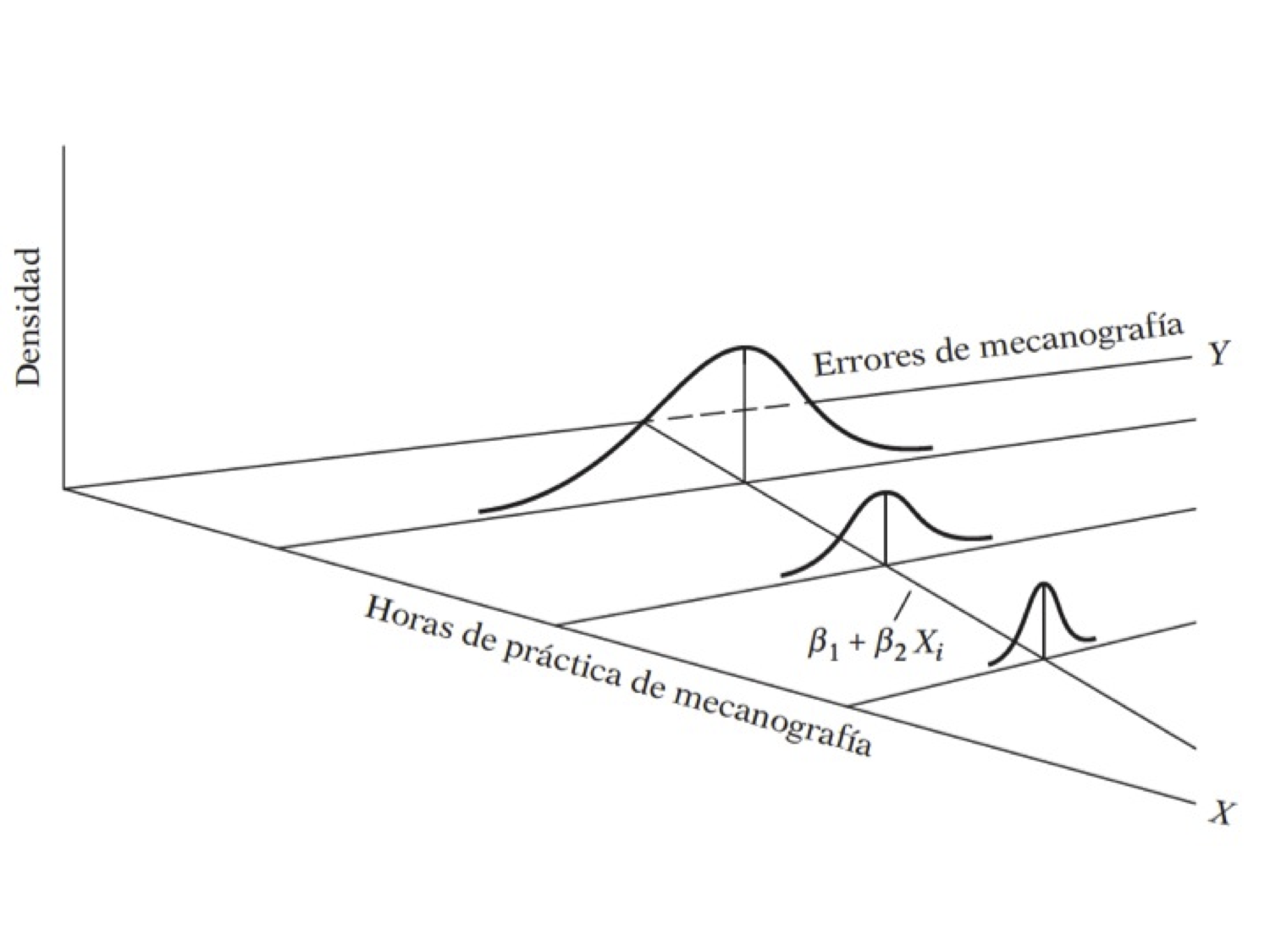
Técnicas de recolección de datos: si la técnica mejora, es probable que la varianza se reduzca.
Datos atípicos o aberrantes: Sensibilidad en las estimaciones
Especificaciones del modelo: Omisión de variables importantes en el modelo.
Asimentría: Surge a partir de la distribución de una o más regresoras en el modelo. Ejemplo: Distribución del ingreso generalmente inequitativo
6.3.2.1. ¿Cómo detectarla?#
Método gráfico
Veamos las pruebas de detección en un ejemplo
Abrir la base de datos wage1 de Wooldrigde
uu = "https://raw.githubusercontent.com/vmoprojs/DataLectures/master/WO/wage1.csv"
datos = pd.read_csv(uu,header=None)
datos.columns = ["wage",  "educ",  "exper",  "tenure",
               "nonwhite","female","married",
               "numdep","smsa","northcen","south",
               "west","construc","ndurman","trcommpu",
               "trade","services","profserv","profocc",
               "clerocc","servocc","lwage","expersq",
               "tenursq"]
datos["casados"] = (1-datos.female)*datos.married  # female 1=mujer  married=1 casado
datos["casadas"] = (datos.female)*datos.married
datos["solteras"] = (datos.female)*(1-datos.married)
datos["solteros"] = (1-datos.female)*(1-datos.married)
Correr el modelo $\( lwage = \beta_{0}+\beta_{1}casados+\beta_{2}casadas+\beta_{3}solteras +\beta_{4}educ+\beta_{5}exper+\beta_{6}expersq +\beta_{7}tenure+\beta_{8}tenuresq+u_{i} \)$
Hacer un gráfico de los valores estimados y los residuos al cuadrado
6.3.2.2. Prueba de Breusch Pagan#
Correr un modelo de los residuos al cuadrado regresado en las variables explicativas del modelo global.
het_breuschpagan: si el pvalor es inferior a \(0.05\),Ho: Homocedasticidad
El códgio en Python sería:
ajuste1 = stm.ols("lwage~casados+casadas+solteras+educ+exper+expersq+tenure+tenursq",data = datos)

print(ajuste1.fit().summary())
residuos = ajuste1.fit().resid
sqresid = residuos**2
y_techo = ajuste1.fit().fittedvalues
#https://www.statsmodels.org/stable/generated/statsmodels.regression.linear_model.RegressionResults.html#statsmodels.regression.linear_model.RegressionResults
plt.scatter(y_techo,sqresid)
plt.gca().update(dict(title='', xlabel='y techo', ylabel='Residuos'))
                            OLS Regression Results
==============================================================================
Dep. Variable:                  lwage   R-squared:                       0.461
Model:                            OLS   Adj. R-squared:                  0.453
Method:                 Least Squares   F-statistic:                     55.25
Date:                Wed, 16 Apr 2025   Prob (F-statistic):           1.28e-64
Time:                        04:05:11   Log-Likelihood:                -250.96
No. Observations:                 526   AIC:                             519.9
Df Residuals:                     517   BIC:                             558.3
Df Model:                           8
Covariance Type:            nonrobust
==============================================================================
                 coef    std err          t      P>|t|      [0.025      0.975]
------------------------------------------------------------------------------
Intercept      0.3214      0.100      3.213      0.001       0.125       0.518
casados        0.2127      0.055      3.842      0.000       0.104       0.321
casadas       -0.1983      0.058     -3.428      0.001      -0.312      -0.085
solteras      -0.1104      0.056     -1.980      0.048      -0.220      -0.001
educ           0.0789      0.007     11.787      0.000       0.066       0.092
exper          0.0268      0.005      5.112      0.000       0.017       0.037
expersq       -0.0005      0.000     -4.847      0.000      -0.001      -0.000
tenure         0.0291      0.007      4.302      0.000       0.016       0.042
tenursq       -0.0005      0.000     -2.306      0.022      -0.001   -7.89e-05
==============================================================================
Omnibus:                       15.526   Durbin-Watson:                   1.785
Prob(Omnibus):                  0.000   Jarque-Bera (JB):               32.182
Skew:                          -0.062   Prob(JB):                     1.03e-07
Kurtosis:                       4.205   Cond. No.                     4.86e+03
==============================================================================

Notes:
[1] Standard Errors assume that the covariance matrix of the errors is correctly specified.
[2] The condition number is large, 4.86e+03. This might indicate that there are
strong multicollinearity or other numerical problems.
[Text(0.5, 1.0, ''), Text(0.5, 0, 'y techo'), Text(0, 0.5, 'Residuos')]
# Test para ver si hay heterocedasticidad
ajuste2 = stm.ols("sqresid~casados+casadas+solteras+educ+exper+expersq+tenure+tenursq",data = datos)
print(ajuste2.fit().summary())
                            OLS Regression Results
==============================================================================
Dep. Variable:                sqresid   R-squared:                       0.025
Model:                            OLS   Adj. R-squared:                  0.010
Method:                 Least Squares   F-statistic:                     1.662
Date:                Wed, 16 Apr 2025   Prob (F-statistic):              0.105
Time:                        04:05:12   Log-Likelihood:                -55.216
No. Observations:                 526   AIC:                             128.4
Df Residuals:                     517   BIC:                             166.8
Df Model:                           8
Covariance Type:            nonrobust
==============================================================================
                 coef    std err          t      P>|t|      [0.025      0.975]
------------------------------------------------------------------------------
Intercept      0.0503      0.069      0.729      0.466      -0.085       0.186
casados       -0.0487      0.038     -1.276      0.202      -0.124       0.026
casadas       -0.0515      0.040     -1.291      0.197      -0.130       0.027
solteras       0.0042      0.038      0.108      0.914      -0.071       0.080
educ           0.0038      0.005      0.834      0.405      -0.005       0.013
exper          0.0101      0.004      2.790      0.005       0.003       0.017
expersq       -0.0002   7.61e-05     -2.720      0.007      -0.000   -5.75e-05
tenure         0.0005      0.005      0.102      0.919      -0.009       0.010
tenursq      8.67e-05      0.000      0.544      0.587      -0.000       0.000
==============================================================================
Omnibus:                      624.508   Durbin-Watson:                   1.947
Prob(Omnibus):                  0.000   Jarque-Bera (JB):            68316.816
Skew:                           5.530   Prob(JB):                         0.00
Kurtosis:                      57.725   Cond. No.                     4.86e+03
==============================================================================

Notes:
[1] Standard Errors assume that the covariance matrix of the errors is correctly specified.
[2] The condition number is large, 4.86e+03. This might indicate that there are
strong multicollinearity or other numerical problems.
print(ajuste2.fit().fvalue)# Estaditistico F
print(ajuste2.fit().f_pvalue)# ovalor de F
1.66213192035643
0.1049935552326956
import statsmodels.stats.api as sms
from statsmodels.compat import lzip
nombres = ['Lagrange multiplier statistic', 'p-value',
         'f-value', 'f p-value']

resultado = sms.het_breuschpagan(ajuste1.fit().resid,ajuste1.fit().model.exog)
lzip(nombres, resultado)
[('Lagrange multiplier statistic', 13.189307860806634),
 ('p-value', 0.10549999125863747),
 ('f-value', 1.66213192035643),
 ('f p-value', 0.1049935552326956)]
Para estimar errores robustos (como robust en stata):
ajuste1.fit().HC0_se
Intercept    0.108528
casados      0.056651
casadas      0.058265
solteras     0.056626
educ         0.007351
exper        0.005095
expersq      0.000105
tenure       0.006881
tenursq      0.000242
dtype: float64